Discrete Random Variables and Probability Distributions
Random variables are mathematical variables, having a specific domain (set of possible values). All instances (values) of the random variables occur by chance. They can be interpreted as elementary events. Acording to Wikipedia, a probability-theoretical definition states that "a random variable is understood as a measurable function defined on a probability space that maps from the sample space to the real numbers." [6]
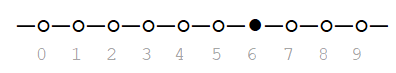
A discrete random variable has a domain made of countable numbers (" ... finitely many or countably infinitely many different values." [1]). Typically, it results from counting procedures (experiments). Here the sample space is mapped to a set (or subset) of integers, ℤ = (0,1,2,...,∞). The domain of the variable can be finite (bounded) or infinite (unbounded). For example, the number of Heads, coming up in an experiment of flipping a coin 9 times, is a discrete random variable with its domain consisting of numbers 0,1,2,...,9. However, theoretically speaking, the number of potholes on Route 20, between Springfield and Framingham has an unbounded domain of numbers 0,1,2,..., ∞, which is ℤ. The discrete variable can be visualized as a collection of [discrete] points marked up on the X-axis. The former example can be described in the following way:

To say that the number of Heads is equal to 6 (X = 6) can be visualized as:
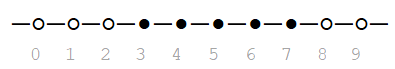
For the number of Heads to be between 3 and 7, we have:
One has to be very careful about interpreting discrete random variables. Paying attention to the limits is critical.
For example, relation X > 5 implies that X is to take on 6, 7, 8, or 9 (the value 5 of is exclusive):
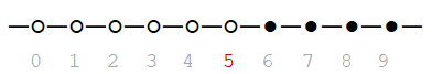
For example, relation X > 5 implies that X is to take on 6, 7, 8, or 9 (the value 5 of is exclusive):
Whether or not a limit is inclusive or exclusive makes a significant difference in assessing probabilities of discrete variables.
A probability distribution defines [exhaustively] chances at which each value (or collection of values) of a random variable occurs. It is defined as a set of pairs (xk, pk), where pk = P(X = xk). It reads as p sub k is the probability of random variable X happening at the level of x sub k.
We can also say that the probabilities are defined by a mathematical function, f(xk), which maps each value, xk, to its probability, pk. Thus f(xk) = P(X = xk). Function f(xk) is referred to as a density or probability mass function. We can also called this function as a point probability function, since it represents the probability of just one value (point on the X-axis).
Note that sometimes we will use a shortcut notation: P(X = xk) = P(xk) or just P(x) if the interpretation of the random variable is clear. If index k matches a value of random variable X, the the probability of X to be equal to k is simply denoted as pk, P(X = k) = pk.
In order for a function, f(xk), to be a probability density function, the following condition must be satisfied:
(1) Each value of the function must be a probability: 0 ≤ f(xk) ≤ 1.
(2) All values of the function must add up to 1: f(x1) + f(x2) +...+ f(xn) = 1.
Notice that for an infinite domain we have: f(x1) + f(x2) + ... + f(x∞) = 1
A very handy function, F(xk), denotes the cumulative probability, F(xk) = P(X ≤ xk) = f(x1) + f(x2) + ...+ f(xk). Because of this additive property and discrete nature, the cumulative probability function can also be defined as F(xk) = F(xk-1) + f(xk). The cumulative probability function, (for short—probability function) can be used to assess interval probabilities. For example (be careful about handling the end points). The following are typical discrete probability patterns:
Pattern 1. The cumulative probability of the random variable taking on a value up to point xk:
P(X ≤ xk) = P(X ≤ xk) = F(xk)
P(X ≤ xk) = P(X ≤ xk) = F(xk)
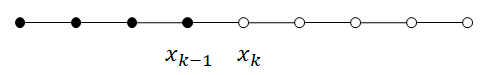
Pattern 2. The cumulative probability of the random variable taking on a value less than (below point) xk:
P(X < xk) = P(X ≤ xk-1) = F(xk-1)
P(X < xk) = P(X ≤ xk-1) = F(xk-1)
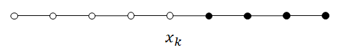
Pattern 3. The probability of the random variable taking on a value above point xk:
P(X > xk) = 1 - P(X ≤ xk) = 1 - F(xk)
This pattern is complementary to Pattern 1. Not Pattern 1 ≡ Pattern 3.
1 - F(xk) = 1 - F(xk)
P(X > xk) = 1 - P(X ≤ xk) = 1 - F(xk)
This pattern is complementary to Pattern 1. Not Pattern 1 ≡ Pattern 3.
1 - F(xk) = 1 - F(xk)
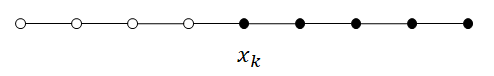
Pattern 4. The probability of the random variable taking on a value at or above point xk:
P(X ≥ xk) = 1 - P(X < xk) = 1 - P(X ≤ xk-1) = 1 - F(xk-1)
This pattern is complementary to Pattern 2. Not Pattern 2 ≡ Pattern 4.
1- F(xk-1) = 1 - F(xk-1)
P(X ≥ xk) = 1 - P(X < xk) = 1 - P(X ≤ xk-1) = 1 - F(xk-1)
This pattern is complementary to Pattern 2. Not Pattern 2 ≡ Pattern 4.
1- F(xk-1) = 1 - F(xk-1)
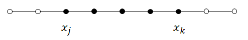
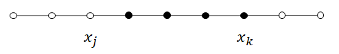
Pattern 5. The probability of the random variable taking on a value between points xj and xk (inclusively):
P(xj ≤ X ≤ xk) = P(X ≤ xk) - P(X ≤ xj-1) = F(xk) - F(xj-1)
P(xj ≤ X ≤ xk) = P(X ≤ xk) - P(X ≤ xj-1) = F(xk) - F(xj-1)
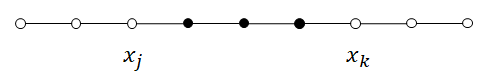
Pattern 6. The probability of the random variable taking on a value greater than xj and less than or equal to xk:
P(xj < X ≤ xk) = P(X ≤ xk) - P(X ≤ xj) = F(xk) - F(xj)
P(xj < X ≤ xk) = P(X ≤ xk) - P(X ≤ xj) = F(xk) - F(xj)
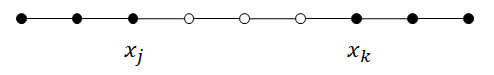
Pattern 7. The probability of the random variable taking on a value between points xj and xk (exclusively - the end point are not considered):
P(xj < X < xk) = P(X ≤ xk-1) - P(X ≤ xj = F(xk-1) - F(xj)
P(xj < X < xk) = P(X ≤ xk-1) - P(X ≤ xj = F(xk-1) - F(xj)
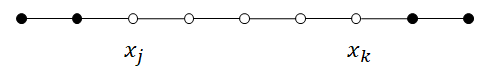
Pattern 8. The probability of the random variable taking on a value up to point xj or at least xk (xj < xk):
P(X ≤ xj or X ≥ xk) = P(X ≤ xj) + P(X ≥ xk) = P(X ≤ xj) + 1 - P(X ≤ xk-1) = F(xj) + 1 - F(xk-1)
This pattern is complementary to Pattern 7. Not Pattern 7 ≡ Pattern 8.
1- (F(xk-1) - F(xj)) = F(xj) + 1 - F(xk-1)
P(X ≤ xj or X ≥ xk) = P(X ≤ xj) + P(X ≥ xk) = P(X ≤ xj) + 1 - P(X ≤ xk-1) = F(xj) + 1 - F(xk-1)
This pattern is complementary to Pattern 7. Not Pattern 7 ≡ Pattern 8.
1- (F(xk-1) - F(xj)) = F(xj) + 1 - F(xk-1)
Pattern 9. The probability of the random variable taking on a value less than xj or greater than xk (xj < xk):
P(X < xj or X > xk) = P(X < xj) + P(X > xk) = P(X ≤ xj-1) + 1 - P(X ≤ xk) = F(xj-1) + 1 - F(xk)
This pattern is complementary to Pattern 5. Not Pattern 5 ≡ Pattern 9.
1 - (F(xk) - F(xj-1)) = F(xj-1) + 1 - F(xk)
P(X < xj or X > xk) = P(X < xj) + P(X > xk) = P(X ≤ xj-1) + 1 - P(X ≤ xk) = F(xj-1) + 1 - F(xk)
This pattern is complementary to Pattern 5. Not Pattern 5 ≡ Pattern 9.
1 - (F(xk) - F(xj-1)) = F(xj-1) + 1 - F(xk)
Q & A - Discrete Probability
How to derive a point probability from cumulative probabilities? Hint: Express f(xk) in terms of F(xk) and F(xk-1). 
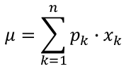
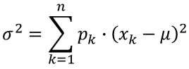
The expected value, μ, of a discrete random variable X over its domain {xk, k=1,2,...,n}, having the probability distribution {pk, k=1,2,...,n}, is the probability-weighted average of the values of this random variable. The variance is a probability-weighted average of the squared differences between the values and their expected value.
| Expected Value, E(X) | Variance, Var (X) |
 |  |
Notice that the standard deviation, σ, is the square root of the variance, σ2.
During the last winter season, store Music Payers reported the following weekly sales: 0 guitars - 5% of the time, 1 guitar - 7% of the time, 2 guitars - 12% of the time, 3 guitars - 20% of the time, 4 guitars - 32% of the time, 5 guitars - 18% of the time, and 6 guitars -6% of the time.
What is the expected value of the weekly sales?
This distribution deals with a discrete random variable, X, having domain of integers (0,1,2,3,4,5,6). Since all the percentages are non-negative, having the total sum of 100%, they can be interpreted as an empirical, discrete probability distribution:
|
The Expected Value:
μ = 0.05 · 0 + 0.07 · 1 + 0.12 · 2 + 0.20 · 3 + 0.32 · 4 + 0.18 · 5 + 0.06 · 6 = 3.45
The Variance:
σ2 = 0.05 · (0-3.45)2 + 0.07 · (1-3.45)2 + 0.12 · (2-3.45)2 + 0.20 · (3-3.45)2 + 0.32 · (4-3.45)2 + 0.18 · (5-3.45)2 + 0.06 · (6-3.45)2 = 3.45
The Standard Deviation:
σ = √3.45 ≅ 1.4925 ≅ 1.5
The expected value (mean) of the weekly-sales quantity is 3.45 guitars.
On average, this quantity deviates from the mean by approximatly 1.5 guitars. |
Spreadsheet Solution
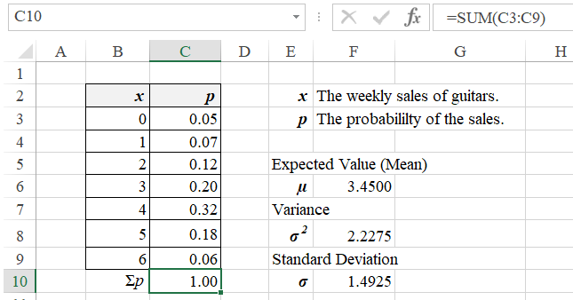
Formulas:
C10:=SUM(C3:C9)
F6: =SUMPRODUCT(B3:B9,C3:C9)
F8: =SUMPRODUCT(C3:C9,(B3:B9-F6)^2)
F10:=SQRT(F8)
This spreadshet solution is also available as an Excel workbook.
R Solution
# The domain of the random sales quantities.
x = c(0,1,2,3,4,5,6)
# The probability distribution of the sales quantities.
p = c(0.05,0.07,0.12,0.2,0.32,0.18,0.06)
# The Expected Value (Mean).
mu = as.numeric(p %*% x)
mu
[1] 3.45
# The Variance.
var = as.numeric(p %*% (x-mu)^2)
var
[1] 2.2275
# The Standard Deviation.
stdev = sqrt(var)
stdev
[1] 1.492481
Mathematical Models of Selected Discrete Random Variables
The Guitar Sales case shows an example of an empirical random variable and its distribution. In this section the following mathematical models of discrete random variables are presented: Binary, Binomial, and Poisson.
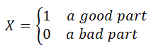
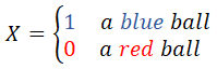
A Binary random variable, referred also as Bernoulli variable [3, X, has two instances: 1 or 0:

Value 1 is frequently mapped to an event that results in success and 0 — to failure. Traditionally, the probability for X = 1 (success) is denoted by letter p and for X = 0 (failure) — by q.
Since events success and failure are disjoint and complementary, we have: q = 1 - p. Both p and q are non-negative and they add up to 1, p + q = p + 1 - p = 1.
P(X = 1) = p
P(X = 0) = q = 1 - p
The Binary variable represents an outcome of a simple experiment, returning randomly one of two [opposite] outcomes. A part being inspected may be good (1) or bad (0). A ball, selected from a jar, containing red and blue balls, will be either red (1) or blue (0). A system may be in an operational (1) state or in a defective (0) state. Etc., etc.
Expected Value
The expected value, μ, of the Binary variable is equal to p.
E(X) = μ = p·1 + q·0 = p
Variance
The variance, σ2, of the Binary variable is equal to p·(1-p).
σ2= p·(1 - μ)2 + q·(0 - μ)2= p·(1 - p)2 + (1-p)·(0 -p)2 = p·(1 - p)2 + (1 - p)·p2 = (1 - p)·( p·(1 - p) + p2) =
= (1 - p)·( p - p2 + p2) = (1 - p)·p
Standard Deviation
The standard deviation, σ, of the Binary variable is equal to the square root of p·(1-p).
Example - Binary
One part is selected from a shipment of 200 parts. The supplier's proportion of defective parts has been 1.5% so far. Define a Binary variable for this situation, assuming that 1 is assigned to a good part (success) and 0 to a bad part (failure). What is the probability of one selected part to be good or bad?
Solution
The random variable, representing the two opposite states of a part, is a Binary variable, X, with X = 1 for success (a good part) or X = 0 for failure (a bad part). Since the proportion of the defective parts is 1.5% and failure is attributed to defective parts, then q = 0.015. Thus p = 1 - q = 0.985; P(X = 1) = p = 0.985, P(X = 0) = q = 0.015.
Alternative "is good part (1) or bad part (0)" is a certain event since events good and bad are disjoint and complementary.
Thus P(X = 1 or X = 0) = P(X = 1) + P(X = 0) = p + q = 0.985 + 0.015 = 1.
Thus P(X = 1 or X = 0) = P(X = 1) + P(X = 0) = p + q = 0.985 + 0.015 = 1.
Exercise - Binary
A Jar contains 2 blue and 3 red balls. The balls are of the identical size, texture, and weight. Define a Binary variable for selecting a blue ball. For this variable, calculate the expected value, variance, and standard deviation. What is the probability that in two independent draws (with replacement) each of the two drawn balls will be blue.
Solution:
There are only two exclusive and complementary events: blue, red. Thus we can define a Binary variable, assigning 1 to blue, or 0 to red:
There are only two exclusive and complementary events: blue, red. Thus we can define a Binary variable, assigning 1 to blue, or 0 to red:
There are 2 + 3 = 5 balls in the Jar. Having 2 blue balls out of 5 total number of balls makes the probability of selecting a blue ball equal to 2/5, P(X = 1) = 2/5 = 0.4.
The expected value, E(X) = μ = p = 0.4.
The variance, Var(X) = σ2 = p · (1 - p) = 0.4 · 0.6 = 0.24.
The standard deviation, σ = √0.24 ≈ 0.49.
The expected value, E(X) = μ = p = 0.4.
The variance, Var(X) = σ2 = p · (1 - p) = 0.4 · 0.6 = 0.24.
The standard deviation, σ = √0.24 ≈ 0.49.
Since the 2 balls are drawn independently and with replacement, each of the drawings can be treated as a replication of outcomes of identical Binary variables.
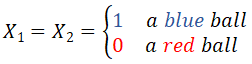
Thus, the probability of getting two blue balls in two independent drawings with replacement fits into the Law of Multiplication with Independent Events:
P(X1 = 1 and X2 = 1) = p · p = 0.4 · 0.4 = 0.16.
There is 16% chance that the two selected balls will be blue.
Spreadsheet Solution:
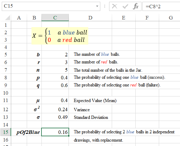
Formulas:
C7: =SUM(C5:C6)
C8: =C5/C7
C9: =1-C8
C11: =C8
C12: =C8*C9
C13: =SQRT(C12)
c15: =C8^2
C7: =SUM(C5:C6)
C8: =C5/C7
C9: =1-C8
C11: =C8
C12: =C8*C9
C13: =SQRT(C12)
c15: =C8^2
Download a solution Workbook.
R Solution:
# The number of blue balls.
b = 2
# The number of red balls.
r = 3
# The total number of the balls in the Jar.
n = b + r
# The probability of selecting one blue ball (success).
p = b/n
p
[1] 0.4
# The probability of selecting one red ball (failure).
q = 1 - p
q
[1] 0.6
# Expected Value, Variance, and Standard Deviation
mu = p
mu
[1] 0.4
var = p*(1-p)
var
[1] 0.24
stdev = sqrt(var)
stdev
[1] 0.4898979
# The probability of selecting 2 blue balls in 2 independent drawings, with replacement.
pOf2Blue = p^2
[1] 0.16
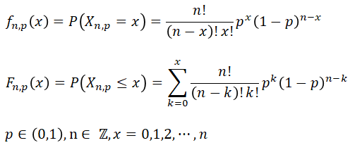
A Binomial random variable, Xn,p, has n+1 instances: 0,1,2, ..., n. It returns randomly the number of successes in a series of n independent trials, where the probability of success in each trial is constant p [4]. Notice that the Binomial variable can be modeled as a sum of n independent Binary variables, each having the probability of success, P(Xn,p = 1), equal to p. In order for a random variable to follow a Binomial probability distribution, it must meet the following requirements:
- The Binomial experiment consists of n independent and homogeneous trials.
- Each trial results in one of two possible outcomes: success or failure.
- The probability, p, of success, is fixed in each of the trials. Since failure is a complementary event, its probability is q = 1-p.
A single trial in the Binomial experiment fits perfectly the Binary model.
The domain of the variable is an ordered set of integers 0, 1 through n:
Xn,p ∈ {0, 1, 2, ..., n}
In a series of n trials there may be 0, 1, 2, ...., or n successes.
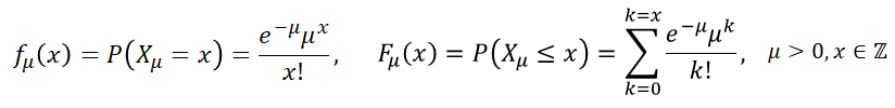
The following formulas define the probablity mass (density) function, fn,p(x), and the cumulative probablity distribution function, Fn,p(x) []:
Spreadsheet functions, doing these probability functions and percentiles, are:
Note: an α's percentile is such a value, x, for which the cumulative probability, P(Xn,p ≤ x), is appoximately equal to α. A similar measure, referred to as a top α's percentile is a value for which P(Xn,p > x) ≈ α.
R functions, doing these probability functions, are:
Binomial Expected Value and Variance / Standard Deviation
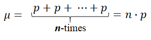
Since the Binomial random variable can be interpreted as a sum of identical and independent Binary variables, the expected value and variance of the Binomial variable is the sum of the expected values and variances of the Binary variable, respectively.
The expected value (mean) of the Binomial variable is the sum of the expected values of the Binary variable:
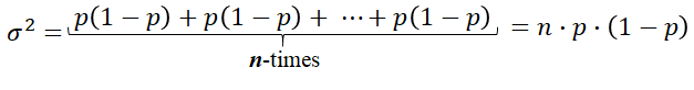
The variance is the average squared deviation from the mean:
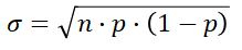
The standard deviation is the square root og the variance:
Example - Binomial
1. What is the probability of getting 3 Heads in an experiment of flipping a fair coin 5 times? Here n=5, x=3, p=0.5.
2. In the same experiment, what is the probability of getting up to 3 Heads?
3. In the same experiment, what is the probability of more than 2 Heads?
4. In the same experiment, what is the 95th percentail for Heads?
5. Also calculate the expected value (mean), variance, and standard deviation.
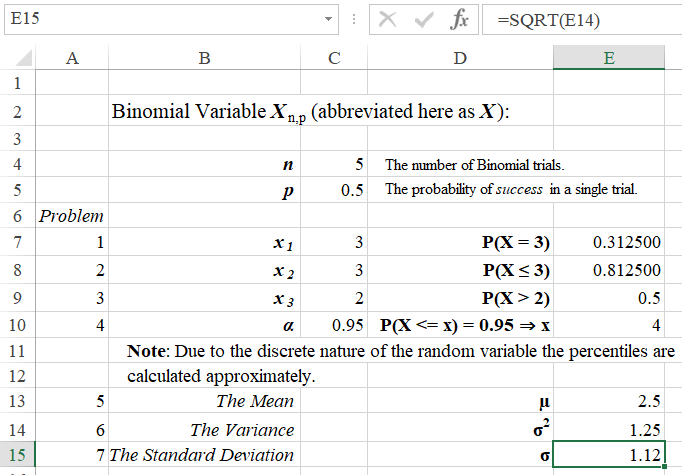
Spreadsheet Solution:
Formulas:
E7: =BINOM.DIST(C7,C4,C5,FALSE)
E8: =BINOM.DIST(C8,C4,C5,TRUE)
E9: =1-BINOM.DIST(C9,C4,C5,TRUE)
E10: =BINOM.INV(C4,C5,C10)
E13: =C5*C4
E14: =C5*(1-C5)*C4
E15: =SQRT(E14)
This spreadshet solution is also available as an Excel workbook.
R Solution
# The number of Binomial trials.
n = 5
# The probability of success.
p = 0.5
# A value of the random variable.
x1 = 3
# The probability of getting x1 Heads.
pof3 = dbinom(x1,n,p)
pof3
[1] 0.3125
# The probability of getting up to x1 Heads.
pof_upto3 = pbinom(x1,n,p)
pof_upto3
[1] 0.8125
# A value of the random variable.
x2 = 2
pof_above2 = pbinom(x2,n,p,lower.tail=FALSE)
pof_above2
[1] 0.5
# A cumulative probability.
alpha = 0.95
# 95th quantile (percentile)
q95th = qbinom(alpha,n,p)
q95th
[1] 4
# Expected Value, Variance, and Standard Deviation
mu = p*n
mu
[1] 2.5
var = p*(1-p)*n
var
[1] 1.25
stdev = sqrt(var)
stdev
[1] 1.118034
Solution Summary:
Given the number of trials (coin flips), n = 5, and the probability of success in a single coin flip (trial), p = 0.5:
| 1 | The probability of getting 3 Heads is 0.3125, P(Xnp = 3) = 0.3125. The Binomial probability mass function is applied (spreadsheet, R). |
| 2 | The probability of getting up to 3 Heads is 0.8125 P(Xnp ≤ 3) = 0.8125. The discrete probability Pattern 1 is utilized. The Binomial cumulative probability function is applied (spreadsheet, R). |
| 3 | The probability of getting more than 2 Heads is 0.5, P(Xnp > 2) = 0.5; The discrete probability Pattern 3 is utilized. The Binomial cumulative probability function is applied (spreadsheet, R). |
| 4 | The 95th percentile is 4, P(Xnp ≤ x) = 0.95 ⇒ x = 4. The Binomial percentile function is applied (spreadsheet, R). Note that because of the discrete nature of this random variable, the 95th percentile is an approximate assessment. If you check the cumulative probability for Xnp = 4, you will get 0.96875. Thus Xnp = 4 is precisely a 96.875th percentile. For Xnp = 3, we get P(Xnp ≤ 3) = 0.8125. Therefore Xnp = 3 is an 81.25th percentile. Lessons learned: percentiles for discrete random variables are closest-neighbor approximates. |
| 5 | The expected value (mean), variance, and statandard deviation are: 2.5, 1.25, 1.12, respectively. On average, the experiment returns 2.5 successes (Heads). The average deviation from this mean is 1.12. Check the definitions of the Mean, Variance, and Standard Deviation. |
Exercise - Binomial Distribution
Seven customers enter Marshalls independently. Historically about 80% of customers, who visit Marshalls, spend $5 or more.
1. What is the probability that no one will spend $5 or more?
2. What is the probability that at least one customer will spend $5 or more?
3. How likely is it that at most three customers will make a purchase?
4. What is the probability that more than five customers will make a purchase?
5. What is the likelihood for 3 to 5 customers to spend 5$ or more.
6. What is an approximate75th percentile of the customers to spend $5 or more.
7. What is the expected value (mean) of the customers spending $5 or more.
8. What is the variance of the customers spending $5 or more.
9. What is the standard deviation of the customers spending $5 or more.
10. What is the expected value (mean) of the customers spending more than $100.
Solution:
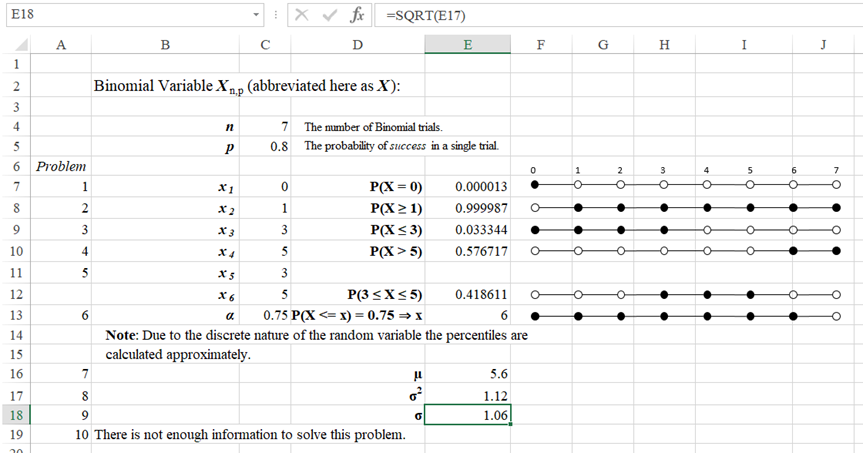
Since the customers enter Marshalls independently, this situation can be modeled, using a Binomial experiment with n = 7 and p = 0.8.
Spreadsheet Solution:
Formulas:
E7: =BINOM.DIST(C7,$C$4,$C$5,FALSE)
E8: =1-BINOM.DIST(C8-1,C4,C5,TRUE)
E9: =BINOM.DIST(C9,$C$4,$C$5,TRUE)
E10: =1-BINOM.DIST(C10,C4,C5,TRUE)
E12: =BINOM.DIST(C12,C4,C5,TRUE)-BINOM.DIST(C11-1,C4,C5,TRUE)
E13: =BINOM.INV(C4,C5,C13)
E16: =C5*C4
E17: =C5*(1-C5)*C4
E18: =SQRT(E17)
R Solution:
# The number of Binomial trials.
n = 7
# The probability of success.
p = 0.8
# A value of the random variable.
x1 = 0
# 1. The probability of no purchase.
pof0 = dbinom(x1,n,p)
sprintf("%.6f",pof0)
[1] "0.000013"
# 2. The probability of 1 or more.
x2 = 1
pof1or_more = pbinom(x2-1,n,p,lower.tail=FALSE)
sprintf("%.6f",pof1or_more)
[1] "0.999987"
# A value of the random variable.
x3 = 3
# 3. The probability of up to 3.
pof_upto3 = pbinom(x3,n,p)
sprintf("%.6f",pof_upto3)
[1] "0.033344"
# 4 The probability of more than 5.
x4 = 5
pof_above5 = pbinom(x4,n,p,lower.tail=FALSE)
sprintf("%.6f",pof_above5)
[1] "0.576717"
# 5 The probability of between 3 and 5 (inclusively).
x5 = 3
x6 = 5
pof_between3and5
pof_between3and5 = pbinom(x6,n,p)-pbinom(x5-1,n,p)
sprintf("%.6f",pof_between3and5)
[1] "0.418611"
# 6 80th percentile
alpha = 0.80
q80th = qbinom(alpha,n,p)
q80th
[1] 7
# 7-9 Expected Value, Variance, and Standard Deviation
mu = p*n
mu
[1] 5.6
var = p*(1-p)*n
var
[1] 1.12
stdev = sqrt(var)
stdev
[1] 1.06
Solution Summary:
This is a Binomial experiment with n = 7 and p = 0.8.
| 1 | The probability that no one will spend $5 or more is 0.000013, P(Xn,p = 0) = 0.000013. This solution use the Binomial probability mass function (spreadsheet, R). |
| 2 | The probability that at least one customer will spend $5 or more is 0.999987, P(Xn,p ≥ 1) = 0.999987. Apply the Binomial cumulative probability function (spreadsheet, R) and discrete probability Pattern 4. |
| 3 | The probability that at most three customers will make a purchase is 0.033344, P(Xn,p ≤ 3) = 0.033344. Apply the Binomial cumulative probability function (spreadsheet, R) and discrete probability Pattern 1. |
| 4 | The probability that more than five customers will make a purchase ($5 or more) is 0.576717, P(Xn,p > 5) = 0.576717. Apply the Binomial cumulative probability function (spreadsheet, R) and discrete probability Pattern 3. |
| 5 | The probability that 3 to 5 customers to spend 5$ or more is 0.418611, P(3 ≤ Xn,p ≤ 5) = 0.418611. Apply the Binomial cumulative probability function (spreadsheet, R) and discrete probability Pattern 5. |
| 6 | The 75th percentile is 4, P(Xnp ≤ x) = 0.75 ⇒ x = 4. Apply the percentile (quantile) function (spreadsheet, R) for the Binomial distribution. |
| 7 | The expected value (mean) of the number of the customers spending $5 or more is 5.6, μ = 5.6. Check the definition of the expected value (μ) for the Binomial distribution. |
| 8 | The variance of the number of the customers spending $5 or more is 1.12, σ2 = 1.12. Check the definition of the variance (σ2) for the Binomial distribution. |
| 9 | The standard deviation of the number of the customers spending $5 or more is 1.06, σ = 1.06. Check the definition of the standard deviation (σ2) for the Binomial distribution. |
| 10 | There is not enough information to solve this problem. |
The Poisson distribution is a probability distribution of a discrete random variable that stands for the number (count) of statistically independent events that occur within a unit of time or space at a constant rate [5]. The rate, μ, happens to be the average number of events that ocur per unit of time or space. Some publications use Greek letter λ to represent this rate.
The domain of such a variable, Xμ, is an ordered set of integers.
Xμ ∈ {0, 1, 2, ..., ∞}
The following formulas define the probablity mass (density) function, fμ(x), and the cumulative probablity distribution function, Fμ(x):
Whether one observes patients arriving at an emergency room, cars driving up to a gas station, decaying radioactive atoms, bank customers coming to their bank, or shoppers being served at a cash register, the streams of such events typically match the Poisson process. The underlying assumption is that the events are statistically independent and the rate, μ, of these events (the expected number of the events per time unit) is constant.
Spreadsheet functions for Poisson probabilities and percentiles (?), are:
R functions for Poisson probabilities and percentiles, are:
Note: an α's percentile is such a value, x, for which the cumulative probability, P(Xn,p ≤ x), is appoximately equal to α. A similar measure, referred to as a top α's percentile is a value for which P(Xn,p > x) ≈ α.
The expected value, μ, of the Poisson variable is equal to the value of the distribution's parameter μ.
E(X) = μ
The variance, σ2, of the Poisson variable is equal to the mean.
Var(X) = σ2 = μ
The standard deviation is the square root of the variance.
StDev(X) = σ = √μ
Example - Poisson
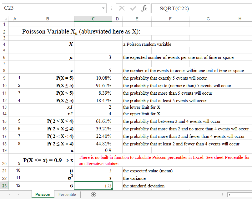
Consider a process in which event occur randomly and independently at a rate of 3 per time unit (μ = 3). Find out the probabilites that (within one time unit):
(1) exactly 5 events will occur;
(2) up to (no more than) 5 events will occur;
(3) more than 5 events will occur;
(4) at least 5 events will occur;
(5) between 2 and 4 events will occur;
(6) more than 2 and no more than 4 events will occur;
(7) more than 2 and fewer than 4 events will occur;
(8) at least 2 and fewer than 4 events will occur.
Also find out:
(9) the 75% percentile of the number of events, a number x for which P(X <= x) = 75%;
(10) the expected value, E(X);
(11) the variance, Var(X) = σ2;
(12) the standard daviation, StDev(X) = σ.
Spreadsheet Solution:
Formulas:
C9: =POISSON.DIST(C8,C6,FALSE)
C10: =POISSON.DIST(C8,C6,TRUE)
C11: =1-C10
C12: =1-POISSON.DIST(C8-1,C6,TRUE)
C15: =POISSON.DIST(C14,C6,TRUE)-POISSON.DIST(C13-1,C6,TRUE)
C16: =POISSON.DIST(C14,C6,TRUE)-POISSON.DIST(C13,C6,TRUE)
C17: =POISSON.DIST(C14-1,C6,TRUE)-POISSON.DIST(C13,C6,TRUE)
C18: =POISSON.DIST(C14-1,C6,TRUE)-POISSON.DIST(C13-1,C6,TRUE)
C21: =C6
C22: =C6
C23: =SQRT(C24)
This spreadshet solution is also available as an Excel workbook. When you open this workbook, also check the Visualization range and sheet Percentile.
R Solution
# Random variable X represents the number of events to occur in one unit of time.
# The expected value of the X.
mu = 3
# A value of the random variable, X.
x = 5
# 1. The probability of 5 events to happen, P(X = 5).
pof5 = dpois(x, mu)
sprintf("%.6f",pof5)
[1] "0.100819"
# 2. The probability of up to 5 events to happen, P(X <= 5).
pofupto5 = ppois(x, mu)
sprintf("%.6f",pofupto5)
pofupto5 = ppois(x, mu)
sprintf("%.6f",pofupto5)
# 3. The probability of more than 5 events to occur, P(X > 5) = 1 - P(X <= 5).
pof_above5 = ppois(x, mu, lower.tail=FALSE)
sprintf("%.6f",pof_above5)
[1] "0.083918"
# Note, the following statement returns the same result:
pof_above5 = 1 - ppois(x, mu)
sprintf("%.6f",pof_above5)
[1] "0.083918"
# 4. The probability of at least 5 events to occur, P(X >= 5) = 1 - P(X <= 4).
pof_atleast5 = ppois(x-1, mu, lower.tail=FALSE)
sprintf("%.6f",pof_atleast5)
[1] "0.184737"
# Note, the following statement returns the same result:
pof_atleast5 = 1 - ppois(x-1, mu)
sprintf("%.6f",pof_atleast5)
[1] "0.184737"
# Limits of the random variable, X.
x1 = 2
x2 = 4
# 5. The probability that between 2 and 4 events will occur (inclusively).
pof_between2and4 = ppois(x2, mu) - ppois(x1-1,mu)
sprintf("%.6f",pof_between2and4)
[1] "0.616115"
# 6. The probability that above 2 and up to 4 events will occur.
pof_above2andupto4 = ppois(x2, mu) - ppois(x1,mu)
sprintf("%.6f",pof_above2andupto4)
[1] "0.392073"
# 7. The probability of above 2 and below 4 events will occur.
pof_above2andbelow4 = ppois(x2-1, mu) - ppois(x1,mu)
sprintf("%.6f",pof_above2andbelow4)
[1] "0.224042"
# 8. The probability that at least 2 and below 4 events will occur.
pof_atleast2andbelow4 = ppois(x2-1, mu) - ppois(x1-1,mu)
sprintf("%.6f",pof_atleast2andbelow4)
[1] "0.448084"
# 9. The 75th percentile (the 3rd quartile).
alpha = 0.75
q75th = qpois(alpha,mu)
q75th
[1] 4
# Notice that q75th = 4 is an approximate value. P(X <= 4) = 0.83
# and P(X <= 3) = 0.65.
# X = 4 is exactly 83th percentile. 83% includes 75% but 65% is not enough.
# ---
# 10-12 Expected Value, Variance, and Standard Deviation
mu
[1] 3
var = mu
var
[1] 3
stdev = sqrt(var)
stdev
[1] 1.73205
Solution Summary:
This is a Poisson process with the average rate μ = 3 (it is expected that 3 events will occur per time unit).
| 1 | The probability that exactly 5 events will occur is 10.08%. The solution is given by the Poisson probability mass function (spreadsheet, R), P(X = 5). |
| 2 | The probability that up to 5 events will occur is 91.61%. The solution is given by the Poisson cumulative probability function (spreadsheet, R), utilizing discrete probability Pattern 1, P(X ≤ 5). |
| 3 | The probability that more than 5 events will occur is 8.39%.The solution is given by the Poisson cumulative probability function (spreadsheet, R), utilizing discrete probability Pattern 3. This solution can also be derived from the previous one (2) by noticing that event "more than 5" is complementary to "up to 5", P(X > 5) = 1 - P(X ≤ 5). |
| 4 | The probability that at least 5 events will occur is 18.47%. The solution is given by the Poisson cumulative probability function (spreadsheet, R), utilizing discrete probability Pattern 4, P(X ≥ 5) = 1 - P(X < 5) = 1 - P(X ≤ 4). |
| 5 | The probability that between 2 and 4 events will occur is 61.61%. The solution is given by the Poisson cumulative probability function (spreadsheet, R), utilizing discrete probability Pattern 5. P( 2 ≤ X ≤ 4) = P(X ≤ 4) - P(X < 2) = P(X ≤ 4) - P(X ≤1). |
| 6 | The probability that more than 2 and no more than 4 events will occur is 39.21%. The solution is given by the Poisson cumulative probability function (spreadsheet, R), utilizing discrete probability Pattern 6. P( 2 < X ≤ 4) = P(X ≤ 4) - P(X ≤ 2). |
| 7 | The probability that more than 2 and fewer than 4 events will occur is 22.40%. The solution is given by the Poisson cumulative probability function (spreadsheet, R), utilizing discrete probability Pattern 7. P( 2 < X < 4) = P(X < 4) - P(X ≤ 2) = P(X ≤ 3) - P(X ≤ 2). |
| 8 | The probability that at least 2 and fewer than 4 events will occur is 44.81%, P( 2 ≤ X < 4) = P(X < 4) - P(X < 2) = P(X ≤ 3) - P(X ≤1) . |
| 9 | The 75th percentile of the number of events, a number x for which P(X ≤ x) = 75%. There is no direct spredsheet function to calculate percentiles (quantiles). R provides an appriximate solution, x = 4., using its q function. |
| 10 | The expected value, E(X) = μ = 3. |
| 11 | The variance, Var(X) = σ2 = μ = 3. |
| 12 | The standard daviation, StDev(X) = σ ≈ 1.7321 |
Exercise - Poisson Distribution
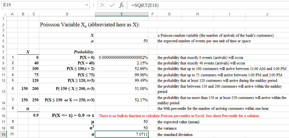
The average number of customers arriving at a bank per one hour, during the midday period (between 11:00 AM and 2:00 PM), is 50. Assume that all arrivals are independent from one another and the average rate applies within any one hour of the period.
1. What is the probability that no one will arrive between 11:00 AM and 12:00 PM?
2. What is the probability that 40 customers will arrive at the bank between 11:00 AM and 12:00 PM?
3. What is the probability that 100 customers will arrive between 11:00 AM and 1:00 PM?
4. How likely is it that at up to 75 customer will arrive between 1:00 PM and 2:00 PM?
5. How likely is it that at least 120 customers will arrive during the midday period?
6. What is the probability that between 100 and 200 customers will arrive within the midday period?
7. How likely is it that no more than 50 or at least 200 customers will arrive within the midday period?
8. Find out the 90th percentile for the number of arriving customers (such a value, x, for which P(X ≤ x) = 0.9).
9-11. Find out the expected value (mean), variance, and standard deviation of the numer of the arriavals within the midday period.
Solution:
The average arrival rate is 50 (μ). It is expected to that 50 customers will arrive in one hour within the midday period (11:00 AM and 2:00 PM).
The average arrival rate is 50 (μ). It is expected to that 50 customers will arrive in one hour within the midday period (11:00 AM and 2:00 PM).
Spreadsheet Solution:
Formulas:
E8: =POISSON.DIST(C8,E5,FALSE)
E9: =POISSON.DIST(C9,E5,FALSE)
E10: =POISSON.DIST(C10,2*E5,TRUE)
E11: =POISSON.DIST(C11,E5,TRUE)
E12: =1-POISSON.DIST(C12-1,3*E5,TRUE)
E13: =POISSON.DIST(C13,3*E5,TRUE)-POISSON.DIST(B13-1,3*E5,TRUE)
E14: =POISSON.DIST(B14,3*E5,TRUE)+1-POISSON.DIST(C14-1,3*E5,TRUE)
E17: =E5
E18: =E5
E19: =SQRT(E18)
This spreadshet solution is also available as an Excel workbook.
R Solution
# Random variable X represents the number of events to occur in one unit of time.
# The expected value of the X.
mu = 50
# A value of the random variable, X.
x = 0
# 1. The probability that exactly 0 events (arrivals) will occur in one hour, P(X = 0).
pof0 = dpois(x, mu)
sprintf("%.22f",pof0)
[1] "0.0000000000000000000002"
# 2. The probability that exactly 40 events (arrivals) will occur in one hour., P(X = 40).
x = 40
pof40 = dpois(x, mu)
sprintf("%.6f",pof40)
[1] "0.021500"
# 3. The probability that up to 100 customers will arrive between 11:00 AM and 1:00 PM.,
# P(X <= 100, t = 2). This probability considers a 2 hour period. Thus the mean rate
# is twice as high as the mean arrival rate per hour.
x = 100
pof_upto100 = ppois(x, 2*mu)
sprintf("%.6f",pof_upto100)
[1] "0.526562"
# 4. The probability that up to 75 customers will arrive between 1:00 PM and 2:00 PM.,
# P(X <= 75).
x = 75
pof_upto75 = ppois(x, mu)
sprintf("%.6f",pof_upto75)
[1] "0.999628"
# 5. The probability that at least 120 customers will arrive during the midday period.
# P(X >= 120, t=3). The mean arrival rate must be trippled.
x = 120
pof_atleast120 = ppois(x-1, 3*mu, lower.tail=FALSE)
sprintf("%.6f",pof_atleast120)
[1] "0.994895"
# Note, the following statement returns the same result:
pof_atleast120 = 1 - ppois(x-1, 3*mu)
sprintf("%.6f",pof_atleast120)
[1] "0.994895"
# 6. The probability that between 150 and 200 customers will arrive within the midday period.
# Limits of the random variable, X.
x1 = 150
x2 = 200
pof_between150and200 = ppois(x2, 3*mu) - ppois(x1-1,3*mu)
sprintf("%.6f",pof_between150and200)
[1] "0.510816"
# 7. The probability that no more than 150 or at least 250 customers will arrive within
# the midday period.
# Limits of the random variable, X.
x1 = 150
x2 = 250
pof_upto150oratleast250 = ppois(x1, 3*mu) + 1 - ppois(x2-1,3*mu)
sprintf("%.6f",pof_upto150oratleast250)
[1] "0.521697"
# 8. the 90th percentile for the number of arriving customers within one hour
alpha = 0.90
q90th = qpois(alpha, mu)
q90th
[1] 59
# Notice that q90th = 59 is an approximate value. P(X <= 59) = 0.907735
# and P(X <= 58) = 0.883609.
# X = 59 is exactly 90.77th percentile. 90.77% includes 90% but 88.36% is not enough.
# ---
# 9-11 Expected Value, Variance, and Standard Deviation
mu
[1] 50
var = mu
var
[1] 50
stdev = sqrt(var)
stdev
[1] 7.07107
Solution Summary:
| μ | The average number of arrivals per hour between 11:00 AM and 12:00 PM is 50. It is applied in the midday interval (11:00 AM - 2:00 PM). |
| 1 | The probability of exactly 0 arrivals in one hour is negligible (0.00000000000000000002%). The Poisson probability mass function is applied (spreadsheet, R). |
| 2 | The probability that exactly 40 arrivals between 11:00 AM and 12:00 PM (one hour) is about 2.15%. Again the Poisson probability mass function is applied (spreadsheet, R).. |
| 3 | The probability that up to 100 customers will arrive between 11:00 AM and 1:00 PM is 52.66%. In this case, the average arrival rate must be doubled because the time interval is 2 hours. The Poisson cumulative-distribution function (for a 2-hour arrival rate) is applied (spreadsheet, R). Also see the cumulative probability distribution Pattern 1. |
| 4 | The probability that up to 75 customers will arrive between 1:00 PM and 2:00 PM is 99.96%. The Poisson cumulative-distribution function (for an 1-hour arrival rate) is applied (spreadsheet, R). Also see the cumulative probability distribution Pattern 1. |
| 5 | The probability that at least 120 customers will arrive during the midday period is 99.49%. Event "at least 120" is complementary to event "up to 119". This is why P(X ≥ 120) = 1 - P(X ≤ 119). In this case, the average arrival rate must be trippled. The time interval is here 3 hours (the midday period). The Poisson cumulative-distribution function (for an 3-hour arrival rate) is applied (spreadsheet, R). Also see the cumulative probability distribution Pattern 4. |
| 6 | The probability that between 150 and 200 customers will arrive within the midday period is 51.08%. Event "between 150 and 200" can also be expressed as "up to 200 but not less than 150 (excluding numbers 0,1,...,149)". Thus P( 150 ≤ X ≤ 200) = P(X ≤ 200) - P(X ≤ 149). Notice that in the world of discrete variables event "less than 150" (X < 150) is equivalent to event "up to 149 (X ≤ 149)". The Poisson cumulative-distribution function (for an 3-hour arrival rate) is applied (spreadsheet, R). Also see the cumulative probability distribution Pattern 5. |
| 7 | The probability that no more than 150 or at least 250 customers will arrive within the midday period. Event "no more than 150 or at least 250" (X <= 150 or X >= 250) is an alernative of two disjoint (non-overlapping) events: "no more than 150" (X <=150), and "at least 250" (X >= 250). Using the formula for alternative and disjoint events, we get: P(X <= 150 or X >= 250) = P(X <= 150) + P(X >= 250). The Poisson cumulative-distribution function (for an 3-hour arrival rate) is applied (spreadsheet, R). Also see the cumulative probability distribution Pattern 8. |
| 8 | The 90th percentile for the number of arriving customers within one hour. There is no direct spreadsheet solution to this problem. Check the workbook solution on sheet Percentile. In R, the quantile (percentile) function for 1 hour is used (R). |
| 8 | The expected value (μ) is equal to the average arrival rate (see μ definition): μ = 50. |
| 10 | The variance (σ2) is the same as μ (see σ2 definition): σ2 = 50. |
| 11 | The standard deviation (σ) is the square root of the variance (see σ definition): σ ≈ 7.0711. |
The Poisson distribution is very popular. Detail presentation and discussion of the Poisson distribution with Google Sheets examples is provided by [2].
References
| [1] | Brilliant (2020). Discrete Random Variables - Definition. Retrieved from. |
| [2] | Letkowski, J., Developing Poisson probability distribution applications in a cloud. Journal of Case Research in Business and Economics, Volume 5, 2012, Editor: Dr. Barry Thornton, (journal, paper). |
| [3] | Wikipedia-Bernoulli (2020). Bernoulli distribution. Retrieved from. |
| [4] | Wikipedia-Binomial (2020). Binomial distribution. Retrieved from. |
| [5] | Wikipedia-Poisson (2020). Poisson Distribution. Retrieved from. |
| [6] | Wikipedia-Random (2020). Random variable. Retrieved from. |