Probability
Individuals often make their decisions based upon their abilities to answer questions such as:
- What are the chances that sales will decrease if we increase prices?
- How likely is a 10%+ increase of demand after a series of TV adds?
- What is the likelihood a new assembly method will increase productivity?
- What is the probability of finishing a project on time (as planned)?
- What are the odds that a new investment will be profitable?
- What is the mortgage client's probability of success?
- Etc., etc.
Probability Axioms, Definitions, and Rules
The Probability Theory is the soul of Statistics. Most of what we learn from statistical studies is done in terms of probabilistic criteria or properties.
It is therefore important that we understand all major pieces and rules of this theory and learn well how they all act and interact together.
The Probability Theory has a very strong mathematical framework. We will focus here on a light-weight presentation and interpretation of this theory.
Readers interested in more formal approach may wish to explore references shown below (References).
1. Definition
We define the probability as a numeric measure, p, of the likelihood of an event to occur.
This measure is a non-negative number:
p ≥ 0
For an event, A,
the probability of this event to happen is denoted as P(A) (read P of A).
Frequently, probabilities are expressed as percentages, for example, P(A) = 0.5 is equivalent to P(A) = 50%.
2. Certainty
The probability of a certain event, S, is equal to 1 (100%):
P(S) = 1
Here, we represent a certain event as the whole probability (sample) space, S. As shown in Random Events,
we can define certain events in many different ways but, one way or the another, they all are equivalent to the sample space.
A complement of the certain event (S) is an imposible event (∅).
P(∅) = 0
3. Additivity
The probability of a union of disjoint events is the sum of the probabilities of the events:
P(A1 ∪ A1 ∪ ... ∪ An) = P(A1) + P(A2) + ... + P(An)
Events Ak, k = 1,2, ..., n, are all mutually exclusive (disjoint).
For every pair of events (Ai, Aj), the probability of the intersection of the events is zero, P(Ai ∩ Aj) = 0, i, j = 1,2, ..., n, i ≠ j.
One has to be very careful when formulating statements about alternative events. Plain language statements, utilizing coordinating-conjunctive words "and", "or", as well as adverb "not", should be interpreted logically. In particular, word "or" is used to specify an alternative, which is used directly to define event unions. We say that an event belongs to a union of events A1,A2,...,An if it belongs to event A1, OR to event A2, etc. As shown in the above Additivity rule, symbol ∪ stands of a union operator. The same rule could also be expressed as:
P(A1 OR A1 OR ... An) = P(A1) + P(A2) + ... + P(An)
Events and their operators are exhaustively explained in section Random Events.
Probability Definitions
1. Frequency (Empirical)
This definition is based on the frequency, f(X), of an event (X) occurring in a sample of size n.
P(X) = f(X) / n
For example, based on a sample of 36 responses to a marketing question "Are you going to buy an iPhone in the next two month?",
{ yes, no, no, maybe, yes, yes, yes, maybe, no, maybe, yes, maybe, yes, maybe, yes, yes, yes, yes, maybe, no, maybe, maybe, maybe, no, maybe, yes, yes, maybe, yes, yes, yes, no, no, yes, yes, yes },
the probability of event X="yes", can be assessed as 18/36, P(X) = 1/2. Response (event) "yes" appears in the sample 18 times out of the total of 36 events (responses). Event "yes" happened 50% of the time.
2. Chance (Theoretical)
If nx is the number of the simple (elementary) events that satisfy (belong to) event X in a sample space, S, and n
is the total number of the simple events in S, then the probability of X is defined as:
P(X) = nx / n
This definition of the probability assumes that all simple events have the same chance to occur.
This definition is also referred to as a priori or classical.
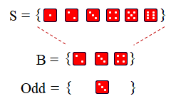
As an example consider an experiment of Rolling a Fair Die with sample space S = {1, 2, 3, 4, 5, 6}.
What is the probability of getting a small number is a single roll? Assume that a small number as not greater than 2.
The event in question is X = {1, 2} so there are 2 simple events that satisfy X.
The total number of all simple events is 6 (the size of S).
Thus the probability of getting a small number in a single roll is 2/6, P(X) = 1/3.
This example is quite simple. More complex cases require more sophisticated methods. Page Counting Rules shows how to handle such cases, utilizing combinatorial formulas.
This example is quite simple. More complex cases require more sophisticated methods. Page Counting Rules shows how to handle such cases, utilizing combinatorial formulas.
3. Subjective (Expert)
An assessment of the probability based on knowledge, expertise, experience, believe, etc.
P(X) = p
For example, Mr. Alan Greenspan says that there is 90% change we will go into a recession next year!
Probability Rules (Laws)
The probability of a union of two events, A and B, is equal to the sum of the probabilities of the events
minus the probability of the intersection of the events:
P(A ∪ B) = P(A) + P(B) - P(A ∩ B)
According to the third axiom, the probability of disjoint events is the sum of the probabilities of the events.
Since the intersection of such events is empty (an impossible event), P(A ∩ B) = 0.
Of a particular interest is the case involving special disjoint events: complementary events, X and Xc.
Since the union of the complementary events constitutes the certain event (sample space S), we get:
P(X ∪ Xc) = P(S) = 1.
Moreover, since the complementary events are disjoint, the probability of their union is the sum of their individual probabilities:
P(X ∪ Xc) = P(X) + P(Xc).
Consequently:
P(X) + P(Xc) = 1
P(X) = 1 - P(Xc)
This law is useful particularly when it easier to calculate the probability of the complementary event. For example, Excel
does not have a [direct] function to calculate the Normal right-tail probabilities, P(X > v). However, function =Norm.Dist(v, μ, σ, TRUE)
returns P(X ≤ v). Since events (X > v) and (X ≤ v) are complementary, we get:
P(X > v) = 1 - Norm.Dist(v, μ, σ, TRUE)
The probability of event A given ( | ) event B has occurred:
P(A | B)
To assess this probability we reduce the sample space to event B.
For example, in Rolling a Die, what is the probability of 3 (A = {3}) if we know that an odd number has come up.
Here B = {1,3,5}. Using the Classic probability definition we have:
P(A | B) = P({3} | {1,3,5}) = 1/3
Two events A and B are said to be independent if:
P(A) = P(A | B)
If the fact that event B has occurred has no impact on the probability of event A, then event A is independent of event B.
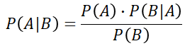
The probability of the intersection (overlap) of events A and B is equal to the product of the probability of event A
and the probability of event B given event A has occurred:
P(A ∩ B) = P(A) ⋅ P(B | A)
If event B is independent of event A, then their "joint" probability is the product of their individual probabilities:
P(A ∩ B) = P(A) ⋅ P(B)
5. Bayes' Theorem
This theorem, also known as Bayes' Law or Formula, provides a way to calculate the [posterior] probability of an event based
on its [prior] (original) probability and based on occurrence of some relevant event.
Let us denote the original event as A and the relevant event as B. The [prior] probability of event A is known, P(A). We want to
find out the [posterior] probability of event A given event B has occurred, P(A | B). In other words, we want to know how much occurrence of event B has influenced the probability of event A to happen. Notice that events A and B occur within the sample space S.
However, after we learn that event B has happened, our focus is on event A in the context of event B.

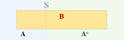
Event B redefines the samples space. Now we are looking at event A with respect to event B rather than within the original
sample space, S.
Notice that event B can also be represented as union of two
intersections of A, Ac and B (event B can occur concurrently with event A or with event Ac):
B = (A ∩ B ) ∪ (Ac ∩ B)
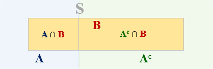
Since events (A ∩ B ) and (Ac ∩ B) are disjoint, the probability of their union can be expressed as
the sum of their probabilities:
P(B) = P(A ∩ B ) + P(Ac ∩ B)
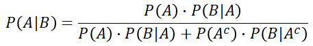
With a little help of the Multiplication Law we can express P(B) as:
P(B) = P(A) ⋅ P(B | A) + P(Ac) ⋅ P(B | Ac)
We can now rewrite the Bayes' Formula, by splitting event B between events A and Ac.
We get an alternative form of the Bayes' Formula.
Let's verify the formulas graphically, using an example in which the sample space, S, consists of 60 identical squares.
Event A is a subset of the space (blue squares). It is made of 25 squares. Obviously the complement of event A, Ac, contains 35 green squares (60 - 25).
Event B occurs as a set of 16 orange squares. What is the probability of event A given event B?
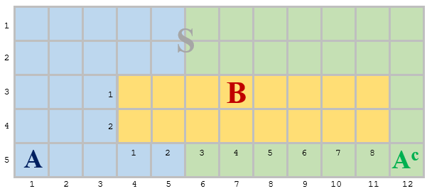
Based on the sizes of the events (sets), we can find out the probabilist: P(A) = 25/60, P(B) = 16/60.
Furthermore, if event A (consisting of 25 squares) has occurred, only 4 squares that belong to A also satisfy event B.
Thus P(B | A) = 4/25.
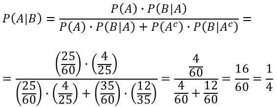
In order to verify the alternative formula we also need the two other probabilities: P(Ac) and P(B | Ac).
Since Ac is a complement of A, then P(Ac) = 1 - P(A) = 1 - 25/60 = 35/60. This result is consistent with the number of squares (35),
contributing to event Ac out of the total of the squares (60) in the sample space (S). If event Ac occurs, then
12 its squares will satisfy event B. Thus P(B | Ac) = 12/35.With all the continuance elements of the alternative formula, we get:
Finally, this problem, P(A | B), can also be solved by analyzing events A and B with respect to the Multiplication Law.
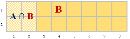
There are 4 squares, satisfying event A that belong to the new sample space (B).
(They are a product of the intersection of events A and B.)
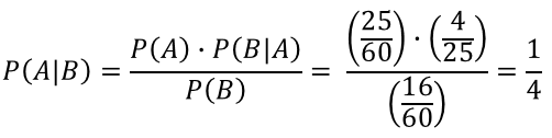
Since event B consists of 16 squares, P(A ∩ B) = 4/16 = 1/4.
In conclusion, this result, P(A | B) = 1/4 = 3/12, should not be surprising. The prior probability, P(A) = 25/60 = 5/12.
However, when event B (a new fact) has occurred, it contributed more to the complement of A (Ac) than to A. Thus, the posterior
probability for event A has decreased (from 5/12 to 3/12).
Examples:
Rolling Dice
Consider an experiment of Rolling a Die (with the sample space S = {1, 2, 3, 4, 5, 6}).
1. What is the probability of number 5 (A = {5}) to come up.

Using the Classical definition, since there is only 1 event in favor of {5} out of 6 possible events, P(A) = 1/6.
Using the Classical definition, since there is only 1 event in favor of {5} out of 6 possible events, P(A) = 1/6.
2. Find the probability of joint events A = {odd} and B = {even} to occur.
Since the events A = {1, 3, 5} and B = {2, 4, 6} are disjoint, their intersection is an impossible event (∅).
Thus P(A ∩ B ) = P(∅) = 0.
Except for being equally likely (1/2), events A and B have nothing in common. If one occurs the other does not.

Moreover, these events are complementary since they are disjoint and their union constitutes the sample space.

The following relations are true about the events:
Except for being equally likely (1/2), events A and B have nothing in common. If one occurs the other does not.
Moreover, these events are complementary since they are disjoint and their union constitutes the sample space.
The following relations are true about the events:
A ∩ B = ∅, A ∪ B = S
P(A ∩ B) = 0, P(A ∪ B) = P(S) = 1
P(A) = 1 - P(B) = 1 - 1/2 = 1/2
P(B) = 1 - P(A) = 1 - 1/2 = 1/2
P(A ∩ B) = 0, P(A ∪ B) = P(S) = 1
P(A) = 1 - P(B) = 1 - 1/2 = 1/2
P(B) = 1 - P(A) = 1 - 1/2 = 1/2
3. Given one of numbers 2, 3, or 4 has been selected (event B = {2, 3, 4} has occurred), what is the probability that it was an odd number.
Here the sample space shrinks to event B. In this space, consisting of 3 elementary events, there is only one odd number ({3}). Thus:
Here the sample space shrinks to event B. In this space, consisting of 3 elementary events, there is only one odd number ({3}). Thus:
P(Odd | B = ) = 1/3
Flipping Coins and Picking Marbles
Now, consider an experiment with coins and marbles in jars. A coin (1 Penny) is flipped twice. Such a flip produces an event, consisting of pairs of heads
(H) and/or tails (T). Jar A contains 4 Red and
3 Blue marbles. Jar B contains 2 Red and
5 Blue marbles. Assume that our experiment has two phases. In Phase 1, the coin is flipped randomly
(independently) twice. Phase 1 returns one of the following, equally likely, events: {HH, HT, TH, TT}.
In Phase 2, a marble is selected from one of the jars, depending on the outcome of Phase 1.
We are interested only on two possible outcomes of Phase 1: {HH} or {HT, TH, TT}. Notice that the latter can also be expressed as
a complement of the former, {HT, TH, TT} = {HT}c. If Phase 1 returns {HH} than a marble is selected from Jar A, otherwise it is selected from Jar B. The following image depicts the experiment structure and its probabilities.
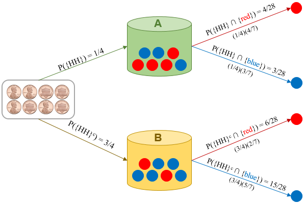
Since in Phase 1, the four possible events are equally likely, then the probability of getting two Heads is 1/4, P({HH}) = 1/4. Notice that this probability can also be calculated as P({H}) ⋅ P({H}) = (1/2)(1/2) = 1/4. The probability of event {H} ∩ {H} is the product of the probabilities since the outcomes of the individual events are produced by independent flips of the coin. (Recall that, for independent events, A and B, we have: P(A ∩ B} = P(A) ⋅ P(B).)
The probabilities of selecting marbles from the jars depend on which jar the marbles are selected from. There are two pathways for selecting a Red marble or Blue marble. The end of each pathway represents a joint event of Phase 1 and Phase 2 outcomes (events), resulting in a Red or Blue marble. Using the Multiplication Law, the probabilities are assessed as follows:
P({HH} ∩ {Red}) = P({HH}) ⋅ P({Red} | {HH}) = (1/4) ⋅ (4/7) = 4/28
(P({Red} | {HH}) = P({Red} | {Jar A})
(P({Red} | {HH}) = P({Red} | {Jar A})
P({HH} ∩ {Red}) = P({HHc}) ⋅ P({Red} | {HHc}) = (3/4) ⋅ (2/7) = 6/28
(P({Red} | {HHc}) = P({Red} | {Jar B})
(P({Red} | {HHc}) = P({Red} | {Jar B})
P({HH} ∩ {Blue}) = P({HH}) ⋅ P({Blue} | {HH}) = (1/4) ⋅ (3/7) = 3/28
(P({Blue} | {HH}) = P({Blue} | {Jar A})
(P({Blue} | {HH}) = P({Blue} | {Jar A})
P({HH} ∩ {Blue}) = P({HHc}) ⋅ P({Blue} | {HHc}) = (3/4) ⋅ (5/7) = 15/28
(P({Blue} | {HHc}) = P({Blue} | {Jar B})
(P({Blue} | {HHc}) = P({Blue} | {Jar B})
Notice that all the above probabilities add up to 1 (4/28 + 6/28 + 3/28 + 15/28 = 1).
4. What is the probability of selecting a Red marble?
From the decision tree, we learn that there are two alternative and disjoint ways of getting a Red marble selected: one via Jar A and
the other via Jar B:
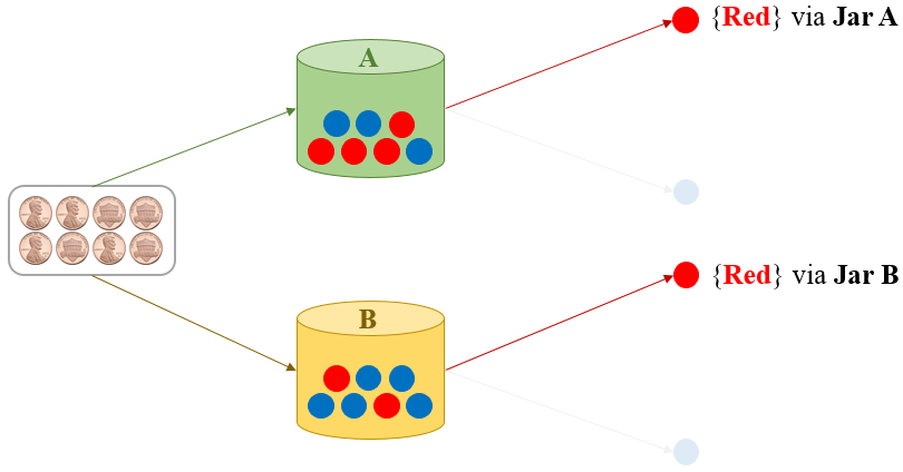
The previous diagram shows the probabilities associated with these alternatives. Thus:
The previous diagram shows the probabilities associated with these alternatives. Thus:
P({Red}) = P({Red via jar A} ∪
{Red via jar B} ) =
P({Red via jar A}) + P({Red via jar B} ) =
4/28 + 6/28 = 10/28 = 5/14
5. What is the probability of selecting a Blue marble in Phase 2
given Phase 1 resulted in HT, TH, or TT?
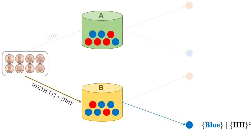
Event {HT,TH,TT} is equivalent to {HH}c. Therefore, if this event has occurred, then automatically Jar B has been selected. There are 5 Blue marbles in jar B out of the total of 7 marbles. Thus:
Event {HT,TH,TT} is equivalent to {HH}c. Therefore, if this event has occurred, then automatically Jar B has been selected. There are 5 Blue marbles in jar B out of the total of 7 marbles. Thus:
P({Blue} | {HT,TH,TT}) = P({Blue} | {HH}c)
= P({Blue} | {Jar B}) = 5 /7
6. A Red marble has been selected.
What is the probability of that it came from Jar A?
This problem is about a conditional probability, P({Jar A} | {Red}).
Applying the base Bayes' Formula, and reusing the above results,
P({Jar A}) = 1/4, P({Red}) = 5/14, we get:
P({Jar A}) = 1/4, P({Red}) = 5/14, we get:
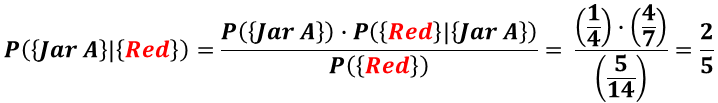
Recall that the a priori probability of selecting Jar A is 1/4. This is the probability of getting 2 Heads in Phase 1,
P({Jar A}) = P({HH}) . With additional knowledge of the fact that a Red
marble has been selected, the posteriori probability, P({Jar A} | {Red}), goes up to 2/5.
A contributing factor for this increased probability is the larger population of Red
marbles in Jar A.
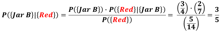
Perform a similar analysis for P({Jar B} | {Red}).

Working with a Contingency Table
A local TV station wanted to learn more about the popularity (preference) of Baseball and Hockey among Men and Women. Forty individuals responded as follows:
| Woman | Baseball | Woman | Baseball | Man | Hockey | Woman | Baseball |
| Man | Hockey | Man | Hockey | Man | Hockey | Woman | Baseball |
| Woman | Hockey | Woman | Baseball | Man | Hockey | Man | Hockey |
| Man | Baseball | Man | Hockey | Woman | Hockey | Man | Baseball |
| Woman | Hockey | Woman | Hockey | Man | Baseball | Woman | Baseball |
| Woman | Baseball | Man | Baseball | Woman | Hockey | Woman | Baseball |
| Woman | Baseball | Man | Hockey | Woman | Baseball | Man | Hockey |
| Man | Hockey | Woman | Baseball | Woman | Baseball | Woman | Baseball |
| Woman | Hockey | Woman | Baseball | Man | Hockey | Man | Baseball |
| Man | Baseball | Man | Hockey | Woman | Baseball | Woman | Baseball |
This survey captured instances of a two-dimensional categorical variable, Sex&Sport, having domain of {Woman&Baseball,
Woman&Hockey, Man&Baseball, Man&Hockey}. Two-dimensional random variables are best summarized by their contingency tables.
The Sex&Sport contingency tables is produced here by counting (cross-tabulating) each element of the domain.
A table (matrix) layout is a convenient representation of such a table. In this case, sixteen Woman-individuals prefer Baseball and six—Hockey.
Six Man-individuals prefer Baseball and twelve—Hockey.
The marginal frequencies show twenty two women and eighteen men participating in the survey. Overall twenty two individuals prefer Baseball and eighteen—Hockey.
By dividing each frequency by the total sample size (40), the contingency table can be expressed as a relative frequency table which is a close as it gets to the probability distribution.
|
|
Events Ac={MPG<20}, Bc={MPG>30} are disjoint. Thus their intersection is empty,
Ac ∩ Bc = ∅
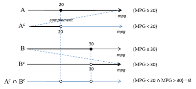
Also in this case, one can apply the De Morgan's law, Ac ∩ Bc = (A ∪ B)c.
Since union A ∪ B = S = {-∞ < MPG < +∞}, its complement is impossible
(A ∪ B)c=∅
Ac ∩ Bc = ∅
Also in this case, one can apply the De Morgan's law, Ac ∩ Bc = (A ∪ B)c.
Since union A ∪ B = S = {-∞ < MPG < +∞}, its complement is impossible
(A ∪ B)c=∅
7. What is the probability for a randomly selected individual to prefer Hockey?
There are 18 out of 40 individuals that prefer Hockey. Thus
P(Hockey) = 18/40 = 9/20 = 0.45
8. What is the probability for a randomly selected individual to be a Woman?
There are 22 women, out of 40 individuals, participating in the survey. Thus
P(Woman) = 22/40 = 11/20 = 0.55
9. Given a randomly selected individual is a Man, what is the probability that he prefers Hockey?
Among 18 men, 12 prefer Hockey. Thus
P(Hockey | Man) = 12/18 = 2/3 ≈ 0.67
10. Are events Man and Hockey independent?
Utilizing the above calculations, the probability of randomly selecting a Man is P(Man) = 1 - P(Woman) = 0.45. Among 18 men, 12 individuals prefer Hockey. Thus P(Hockey | Man) = 12/18 = 2/3. Since P(Man) ≠P(Hockey | Man) the events are not independent.
Exercises
1. Spying on Children [1 p. 153].
According to a global survey of 4,400 parents of children between the ages of 14 to 17, 44% of parents spy on their teen's Facebook account [www.msnbc.com, April 25, 2012]. Assume that American parents account for 10% of all parents of teens with Facebook accounts, of which 60% spy on their teen's Facebook account. Suppose a parent is randomly selected, and the following events are defined:
A = selecting an American parent and
B = selecting a spying parent.
a. Based on the above information, what are the probabilities that can be established?
b. Are the events A and B mutually exclusive and/or exhaustive? Explain.
c. Are the events A and B independent? Explain.
d. What is the probability of selecting an American parent given that she/he is a spying parent? We want to calculate P(A | B).
# The probabity of event A.
pA = 0.10
# The probabity of event B.
pB = 0.44
# The probabity of event B given A, P(B | A).
pBgivenA = 0.60
# The probability of joint events A and B.
pAandB = pBgivenA * pA
pAandB
[1] 0.06
# A condition for independent evants.
pBgivenA == pB
[1] FALSE
# The probability of A given B, P(A | B).
pAgivenB = pAandB / pB
pAgivenB
[1] 0.1363636
An alternative solution, using a contingency table. We can built such a table by cross-referencing the probabilities of events A, Ac vs. B , Bc.
2. Cardiac Arrest vs. Hospital Shift [1 p. 155].
A study in the Journal of the American Medical Association (February 20, 2008) found that
patients who go into cardiac arrest while in the hospital are more likely to die if it happens
after 11 pm. The study investigated 58,593 cardiac arrests that occurred during the day or
evening. Of those, 11,604 survived to leave the hospital. There were 28,155 cardiac arrests
during the shift that began at 11 pm, commonly referred to as the graveyard shift. Of those,
4,139 survived for discharge. The following contingency table summarizes the results of
the study.
| Shift \ Survived | Yes | Not | Total |
| DayEvening | 11604 | 46989 | 58593 |
| Graveyard | 4139 | 24016 | 28155 |
| Total | 15743 | 71005 | 86748 |
a. What is the probability that a randomly selected patient experienced cardiac arrest during the graveyard shift?
b. What is the probability that a randomly selected patient survived for discharge?
c. Given that a randomly selected patient experienced cardiac arrest during the graveyard shift, what is the probability the patient survived for discharge?
d. Given that a randomly selected patient survived for discharge, what is the probability the patient experienced cardiac arrest during the graveyard shift?
e. Are the events "Survived for Discharge" (Yes) and "Graveyard Shift" (Graveyard) independent? Explain using probabilities. Given your answer, what type of recommendations might you give to hospitals?
Solution in R
# Set up a data frame ca (cardiac arrest).
ca = read.table(text="Yes No
11604 46989
4139  24016", header = TRUE)
ca
    Yes    No
1 11604 46989
2  4139 24016
# Add column Total.
ca$Total = rowSums(ca)
ca
    Yes    No Total
1 11604 46989 58593
2  4139 24016 28155
# Add row Total.
ca = rbind(ca, colSums(ca))
ca
    Yes    No Total
1 11604 46989 58593
2  4139 24016 28155
3 15743 71005 86748
# Name rows.
row.names(ca) = c("DayEvening","Graveyard","Total")
ca
Yes No Total DayEvening 11604 46989 58593 Graveyard 4139 24016 28155 Total 15743 71005 86748
a. Solution. What is the marginal probability for event Graveyard, P(Graveyard)?
ca["Graveyard","Total"]/ca["Total","Total"]
[1] 0.3245608
b. Solution. What is the marginal probability for event Yes, P(Yes)?
ca["Total","Yes"]/ca["Total","Total"]
[1] 0.1814797
c. Solution. What is the conditional probability, P(Yes | Graveyard)?
ca["Graveyard","Yes"]/ca["Graveyard","Total"]
[1] 0.1470076
d. Solution. What is the conditional probability, P(Graveyard | Yes)?
ca["Graveyard","Yes"]/ca["Total","Yes"]
[1] 0.2629105
e. Solution. Are events "Graveyard", "Yes" independent? Is P(Graveyard|Yes) = P(Graveyard)?
ca["Graveyard","Yes"]/ca["Total","Yes"] == ca["Graveyard","Total"]/ca["Total","Total"]
[1] FALSE
Glossary
Random Event - an outcome of a Random Experiment (a subset of the set). Also referred to as a compound event.
Probability - a number between 0 and 1 assigned to a random event, with 0 for an impossible event and 1 for a certain event.
References
[1] Jaggia S., Kelly A. Business Statistics: Communicating with Numbers, 3rd Edition, McGraw-Hill Education 2020.
[2] Levine D. M., Stephan D. L., Szabat K. A. Statistics for Managers Using Microsoft Excel, 8/E, Pearson, 2018.