Continuous Random Variables and Probability Distributions
Random variables are mathematical variables, having a specific domain (set of possible values). All instances (values) of the random variables occur by chance. They can be interpreted as elementary events. According to Wikipedia, a probability-theoretical definition states that "a random variable is understood as a measurable function defined on a probability space that maps from the sample space to the real numbers." [Wikipedia-Random Variable]
Continuous random variables have domains made of infinitely many values, and those values are associated with measurements on a continuous scale in such a way that there are no gaps or interruptions within bounded or unbounded intervals.
Brilliant [Continuous Variable] provides a similar definition: "Continuous random variables describe outcomes in probabilistic situations where the possible values some quantity can take form a continuum, which is often (but not always) the entire set of real numbers, ℝ" [Wikipedia-Real Number]. [Wikipedia-Random Variable] says: "Random variables can be ... continuous, taking any numerical value in an interval or collection of intervals (having an uncountable range), via a probability density function that is characteristic of the random variable's probability distribution ... .".
Examples of the domains of continuous random variables are:
- interval (0,1),
- interval (10, 20),

- interval (0, +∞),

- the entire set ℝ of real numbers (- ∞,+ ∞),

- etc.
As mentioned, continuous variable values are results of experiments involving measurements. For example:
- Time T it takes to drive from Springfield - Massachusetts to New York City. This variable has a theoretical domain of positive real number (0, ∞) or (T > 0).
- Weight W of a legal golf ball (maximum 45.93 grams). This variable has a theoretical domain of positive real number (0, 45.93] or (0 < W ≤ 45.93).
- Volume V of gasoline pumped into a 20 gallon tank. This variable has a theoretical domain of positive real number (0, 20] or (0 < V ≤ 20).
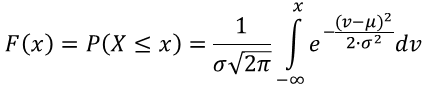
A significant aspect of a continuous random variable, X, is that its probabilities are defined by a [continuous] density function, f(x).
Contrary to the probability mass functions, f(xk) [Wikipedia-Mass-Function], defining the probability distribution of discrete variables, density functions f(x) [Wikipedia-Density], doing a similar job for continuous variables, can't be used to calculate point probabilities. With respect to continuous random variables, their point probabilities are all zeros, P(X = x) = 0. Thus, any assessment of probabities must reference an interval, utilizing a cumulative probability function, F(x) = P(X ≤ x).
Recall that the cumulative probability, F(xk), for a discrete random variable, is the sum of the point probabilities, f(xk), over the domain of the variable, up to point xk.
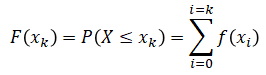
where f(xi) is the probability mass function.
The cumulative probability, F(x), for a continuous random variable, is defined is a similar way, except that the summation is kind of continuous — thus integration:
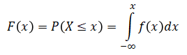
where f(x) is the probability density function.
Fortunately, in most practical cases, such actual integration is not required. Probability software (Excel, R, SAS, etc.) have all build-in functions to deal with the typical probability distributions. Examples of such functions for Empirical, Uniform, Exponential, and Normal distributions are included in the document.
Before getting into the examples let's visualize, side-by-side, cumulative probability distributions for discrete and continuous random variables.
| Discrete | Continuous |
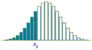 |  |
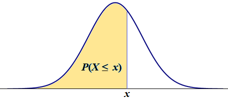
A practical probability of a continuous random variable is an area under the density function. For example:
 |
A good news is that the probability patterns for continuous random variables are simpler than those for the discrete variables.
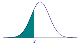
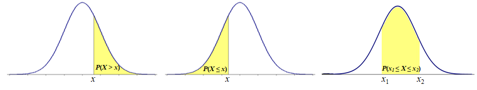
Pattern 1. A Left-tail Probability is the same as the cumulative probability, P(X ≤ x) = F(x):
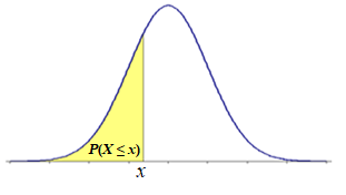
Notice that P(X ≤ x) is that same as P(X < x). It is so because, for continuous random variables, the point probability is equal to zero, P(X = x) = 0. Event (X ≤ x) is equivalent to (X < x) ∪ (X = x), P(X ≤ x) = P[(X < x) ∪ (X = x)]. Since event (X < x) and event (X = x) are disjoint the probability of their union is the sum of the probabilities of the individual events, P[(X < x) ∪ (X = x)] = P(X < x) + P(X = x) = P(X < x) + 0. Thus P(X ≤ x) = P(X < x). This property of the continuous random variables simplifies the probability patterns, reducing them to just basic three patterns.
Notice that P(X ≤ x) is that same as P(X < x). It is so because, for continuous random variables, the point probability is equal to zero, P(X = x) = 0. Event (X ≤ x) is equivalent to (X < x) ∪ (X = x), P(X ≤ x) = P[(X < x) ∪ (X = x)]. Since event (X < x) and event (X = x) are disjoint the probability of their union is the sum of the probabilities of the individual events, P[(X < x) ∪ (X = x)] = P(X < x) + P(X = x) = P(X < x) + 0. Thus P(X ≤ x) = P(X < x). This property of the continuous random variables simplifies the probability patterns, reducing them to just basic three patterns.
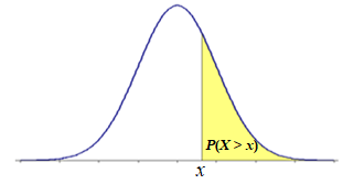
Pattern 2.
A Right-tail Probability is the same as the cumulative probability for the values above point x, P(X > x) = 1 - P(X ≤ x) = 1 - F(x):
Since, for any point x, the left-tail event (X ≤ x) and the right-tail event (X > x) are disjoint and complementary, their probabilities add up to 1, P(X ≤ x) + P(X < x) = 1 (see Law of Addition). Thus P(X > x) = 1 - P(X ≤ x).
Since, for any point x, the left-tail event (X ≤ x) and the right-tail event (X > x) are disjoint and complementary, their probabilities add up to 1, P(X ≤ x) + P(X < x) = 1 (see Law of Addition). Thus P(X > x) = 1 - P(X ≤ x).
Pattern 3. An Interval Probability for the random variable values between two points (x1 ≤ X ≤ x2).
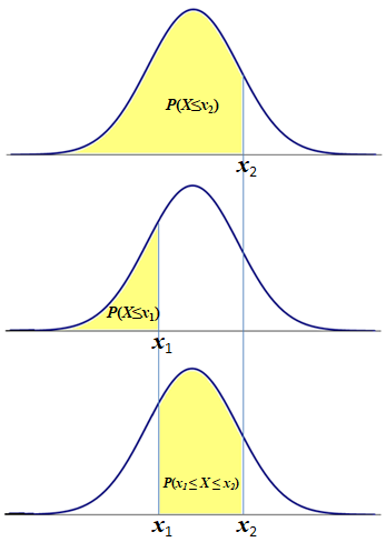
P(x1 ≤ X ≤ x2) = P(X ≤ x2) - P(X ≤ x1) = F(x2) - F(x1):
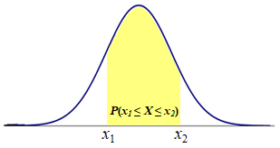
Notice that, if we take the cumulative probability up to point x2, P(X ≤ x2), we will include in it the cumulative probability up to point x1, P(X ≤ x1). By subtracting the latter from the former we get the interval probability"
P(x1 ≤ X ≤ x2) = P(X ≤ x2) - P(X ≤ x1) = F(x2) - F(x1):
Notice that, if we take the cumulative probability up to point x2, P(X ≤ x2), we will include in it the cumulative probability up to point x1, P(X ≤ x1). By subtracting the latter from the former we get the interval probability"
Notice that other patterns can be developed as compositions of the three above patterns.
For example a pattern similar to the discrete Pattern 9, P(X < x1 or X > x2) is a combination of continuous Pattern 1 and Pattern 2, shown above.
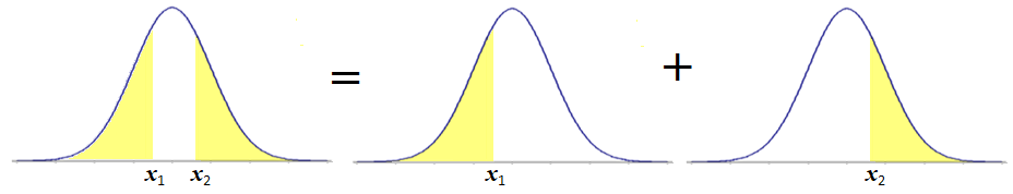
P(X ≤ x1 or X > x2) = P(X ≤x1) + 1 - P(X ≤x2) = F(x1) + 1 - F(x2).
P(X ≤ x1 or X > x2) = P(X ≤x1) + 1 - P(X ≤x2) = F(x1) + 1 - F(x2).
When solving specific problems, all we need is to apply the appropriate function, representing the cumulative probability distribution, F(x).
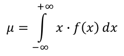
The expected value, μ, of a continuous random variable X over its domain ℝ, having the probability density function f(x), is the probability-weighted average of the values of this random variable. The variance is a probability-weighted average of the squared differences between the values and their expected value. In the case of the continuous random variable, the probability weights are aplied continuosly (integration).
| Expected Value, E(X) | Variance, Var (X) |
 | 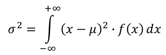 |
Notice that the standard deviation, σ, is the square root of the variance, σ2. Notice that, for the common, continuous random variables, formulas for both μ and σ2 are given.
Mathematical Models of Selected Continuous Random Variables
There are many probability distributions for continuous random varibles.
A good review of the distributions is provided in [Mun]. This section focuses on three popular distributions: Uniform, Exponential, and Normal. Other important distributions (Student-t, χ2, and F, are introduced and applied in the Inferential Statistics pages.
"In probability theory and statistics, the continuous uniform distribution or rectangular distribution is a family of symmetric probability distributions. The distribution describes an experiment where there is an arbitrary outcome that lies between certain bounds. The bounds are defined by the parameters, a and b, which are the minimum and maximum values." [Wikipedia-Uniform]
The uniformly distributed, continuous random variables have bounded-interval domains, [a, b]. Rolling a die produces one of six numbers {1, 2, 3, 4, 5, 6} each having the same (discrete-unform) probability, 1/6. Imagine a wheel with its circumference equal to 6 feet.
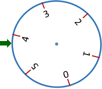
If you trun the wheel with a random force, it will stop eventually, pointing to a number between 0 and 6 (on a continuous scale). This experiment could be thought of as "rolling a continuous die".
If you trun the wheel with a random force, it will stop eventually, pointing to a number between 0 and 6 (on a continuous scale). This experiment could be thought of as "rolling a continuous die".
A Uniform distribution over interval (0,1) is the fundation for many random number generators, built-in programming languages and analytical packages. In spreadsheets, it is implemented by funtion RAND(). In R, function runif(n) is used to generate n uniformly distributed random numbers.
A uniformly distributed random variable, X over interval [a, b], is characterized by its constant density function, f(x):
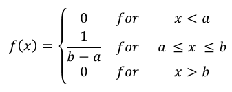
This is a rectangular distribution since the probability is distributed evenly (uniformly) over domain [a, b]:
Notice that the width and height of the rectangle are b-a and 1/(b-a), respectively. Thus the total area of the rectange is (b-a)/(b-a) = 1, making it a valid probability distribution.
This is a rectangular distribution since the probability is distributed evenly (uniformly) over domain [a, b]:
Notice that the width and height of the rectangle are b-a and 1/(b-a), respectively. Thus the total area of the rectange is (b-a)/(b-a) = 1, making it a valid probability distribution.
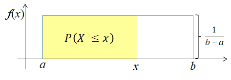
The cumulative probability function, F(x), is the area of the rectangle between the lower limit, a, and point x:
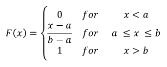
Frequently, acronym cdf is used to represent cumulative distribution function. We will use interchangeably cdf, F(x), P(X ≤ x), or full expression "cumulative probability distribution function". This function is utilized to assess Uniform probabilities.
Frequently, acronym cdf is used to represent cumulative distribution function. We will use interchangeably cdf, F(x), P(X ≤ x), or full expression "cumulative probability distribution function". This function is utilized to assess Uniform probabilities.
The αth percentile (quantile), xα, is the value of the inverse of the cdf, F(xα) = P(X ≤ xα):
P(X ≤ xα)= α ⇒ xα = a + α·(b - a)
This is such a point (x) for which the probability of the random variable to take on any value up to this point is equal to α:
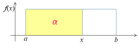
Notice that if F(x) = (x - a)/(b - a) = α then (x - a) = (b - a) · α. This leads to x = a + (b - a) · α.
Notice that if F(x) = (x - a)/(b - a) = α then (x - a) = (b - a) · α. This leads to x = a + (b - a) · α.
The expected value, μ, of the Uniform variable is the value in the middle of interval [a , b].
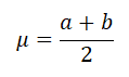
Notice that the Uniform distribution is symmetric. Thus the Uniform mean (μ) is the point of the symmetry.
Notice that the Uniform distribution is symmetric. Thus the Uniform mean (μ) is the point of the symmetry.
The variance of the Uniform variable is one 12th of the squared distance between the limits of interval [a , b]
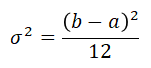
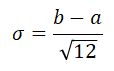
The standard deviation is the square root of the variance:
Example - Uniform
Suppose that the time, T, of completing some task is equally likely between 10 and 20 hours.
| 1 | What is the probability of completing the task in less than 15 hours? |
| 2 | How likely is to complete the task in exactly 15 hours? |
| 3 | What is the probability of completing the task in more than 12 hours? |
| 4 | What is the probability of completing the task in up to 8 hours? |
| 5 | How likely is to complete the task in less to 25 hours? |
| 6 | What is the probability of completing the task in at least 14 hours but not more than 17 hours. |
| 7 | How likely is it to complete the task in less than 12 hours or greater than 16 hours. |
| 8 | What is the 90th percentile of completing the task? |
| 9 | What is the expected value (μ) of the time to complete the task? |
| 10 | What is the variance (σ2) of the time to complete the task? |
| 11 | What is the standard deviation (σ) of the time to complete the task? |
Solution:
This is a simple case. No special software is necessary to solve it. The distribution's parameters are: a = 10, b = 20.
| 1 | x = 15 P(T < x) = F(x) = (x - a)/(b - a) = (15 - 10)/(20 - 10) = 5/10 = 0.5 There is 50% change that the task will be completed in less than 15 hours. This solution uses the Left-tail Probability Pattern. |
| 2 | x = 15 P(T = x) = 0 T is a continuous variable. All point probabilities for such variables are equal to zero. |
| 3 | x = 12 P(T > x) = 1 - P(T ≤ x) = 1 - F(x) = 1 - (x - a)/(b - a) = 1 - (12 - 10)/(20 - 10) = 1 - 2/10 = 0.8 There is 80% chance that the task will be completed in more than 12 hours. This solution uses the Right-tail Probability Pattern. |
| 4 | The probability of completing the task in up to 8 hours is 0, P(T ≤ 8) = 0. Event (T ≤ 8) is impossible. All times are supposed to be between 10 and 20 hours. Also check the definition of the cumulative probability distribution for the Uniform random variable. |
| 5 | The probability of completing the task in less than 25 hours is 1. Although 25 is outside the expected interval [10, 20] but event T ≤ 25 includes the certain event T ≤ 20. Check the definition of the cumulative distribution of the uniform random variable shown above. Also check the definition of the cumulative probability distribution for the Uniform random variable. |
| 6 | This question can be answered, using the Interval Probability Pattern, P(x1 ≤ X ≤ x2), where x1 = 14 and x2 = 17. Using the cdf, we have P(14 ≤ X ≤ 17) = F(17) - F(14) = (17-10)/(20-10) - (14-10)/(20-10) =7/10 - 4/10 = 3/10. Intuitively, we can see that the distance between 14 and 17 is 3. Thus the probability should be 3 units over the total of the 10 units (the length between a and b). Notice that this intuition is valid because we are dealing here with an Uniform distribution. |
| 7 | This question is about two disjoint intervals [10, 12), (16, 20]. It can be answered using the Law of Addition along with the Left-tail Probability Pattern and the Right-tail Probability Pattern. P(X < x1 or X > x2) = P(X < x1) + P(X > x2) = P(X < 12) + P(X > 16) = F(12) + 1 - F(16) = (12-10)/(20-10) + 1- (16-10)/(20-10) = 2/10 + 1 - 6/10 = 6/10. Intuitively, we can see that the length of the first interval is 2 (12 - 10 ) and the length of the second interval is 4 (20 - 16). Thus the probability should be the total langth of the two intervals, 2 + 4 = 6, over 10 (the length between a and b). Notice that this intuition is valid because we are dealing here with an Uniform distribution. |
| 8 | α = 0.9 The αth; percentile of completing the task is a + α · (b - a) = 10 + 0.9 · (20 - 10) = 19. Notice that the cumulative distribution for x = 19 returns 0.9, F(19) = (19 - 10)/(20 - 10) = 9/10. Intuitively, this percentile is a point at the 90% of the total distance between a and b. |
| 9 | The expected value (μ) of the time to complete the task is (a + b)/2 = (10 + 20)/2 = 15 (see definition of μ). |
| 10 | The variance (σ2) of the time to complete the task (b - a)2/12 = (20 - 10)2/12 = 100/12 ≈ 8.333333 (see definition of σ2). |
| 11 | The standard deviation (σ) of the time to complete the task is the square root of the variance, σ ≈ 2.886751. On average, the completion time deviates from the mean (15) by approximately 2.89 (see definition of σ). |
Q & A - Uniform Distribution
The owner of local restaurant Under the Golden Moon has conducted a study that led him to believe that during the last winter season the amount of the potato salad consumed per one customer visit is uniformly distributed between the limits of 250 and 450 grams. Notice that all the following questions are related to one customer's visit. A randomly select customer has just entered the restaurant.
| 1 | What is the probability that the customer will consume more than 500 grams of the salad? |
| 2 | How likely is it for the customer to consume exactly 300 grams of the salad? |
| 3 | What is the probability that the customer will consume up to 400 grams of the salad? |
| 4 | What is the probability that the customer will consume at least 300 grams of the salad? |
| 5 | How likely is it for the customer to consume between 300 and 400 grams of the salad? |
| 6 | What is the probability that the customer will consume no more than 300 and at least 400 grams of the salad? |
| 7 | How likely is it for the customer to consume exactly 300 or more than 350 grams of the salad? |
| 8 | What is the 3rd quartile of the amount of the consumed salad? |
| 9 | What is the expected value (μ) of the amount of the consumed salad? |
| 10 | What is the variance (σ2) of the amount of the consumed salad? |
| 11 | What is the standard deviation (σ) of the amount of the consumed salad? |
"In probability theory and statistics, the Exponential distribution is the probability distribution of the time between events in a Poisson point process, i.e., a process in which events occur continuously and independently at a constant average rate." [Wikipedia-Exponential]
The Exponential probability distribution has many important applications. It is particularily relevant to service-oriented processes. In processes of random and independent events that occur at an average rate (λ), the times between ocurrences of the events is frequently exponentially distributed. For example, the time between arrivals of cars (custmers) at a drive-though services is often exponentially distributed. In many situations, the time it takes to complete service of a customer in a bank, at a gas station, in grocery store, in an emergency room, etc., is exponentially distibuted. With respect to space, the distance between pothols on a road can also be exponentially distibuted.
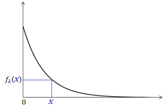
An exponentially distributed, non-negative random variable, Xλ characterized by the following density function, fλ(x):
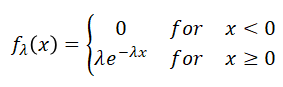 |  |
Paramter λ is referred to as a rate parameter. It represents the average number of events that occur per one time unit (hour, minute, second, etc.).
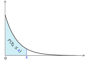
This is an extremly asymmetric distribution. It favors smaller outcomes, closer to zero. Large outcomes are rather rare (less likely).
This is an extremly asymmetric distribution. It favors smaller outcomes, closer to zero. Large outcomes are rather rare (less likely).
The cumulative probability function, Fλ(x), is the area under the density function curve between the lower limit, 0, and point x:
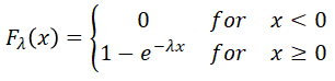 |  |
Exponential vs. Poisson
In a process of independent random events, occuring independently at a fixed average rate (λ), the times between the event ocurrances are exponentially distibuted. Notice that, if you check the definition of the Poisson distribution, with respect to the count of the events, you will realize that we are dealing here with a Poisson process. The following figure shows such a relation between the Poisson and Exponential distributions.
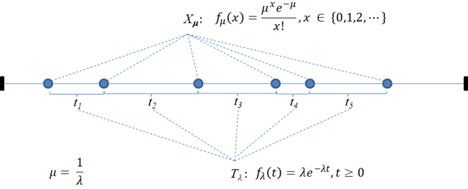
The number of the events (Xμ) is a Poisson random variable. The times (Tλ = t1, t2, ...) are exponentially distributed.
The αth percentile (quantile), xα, is the value of the inverse of the cdf, Fλ(xα) = P(Xλ ≤ xα). This is such a value, xα, for which the cumulative probability is equal to α. In short, we write: P(Xλ ≤ xα) = α then xα is the αth percentile (quantile) or:
P(Xλ ≤ x) = α ⇒ x = xα = -ln(1 - α) / λ.
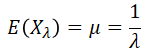
The expected value (mean), μ, of the Exponential variable is the reciprocal of the λ rate.
Notice that the median (xmed) is equal to ln(2)/λ. It is about 70% of the mean With the mode (xmod) being equal to 0, we are dealing here with a very strong asymmetry. The Exponential distribution is extremly right-skewed (positively-skewed).
Notice that the median (xmed) is equal to ln(2)/λ. It is about 70% of the mean With the mode (xmod) being equal to 0, we are dealing here with a very strong asymmetry. The Exponential distribution is extremly right-skewed (positively-skewed).
Q & A - Median & Mode
Why is the median (xmed) for the exponential distribution is equal to ln(2)/λ, and the mode (xmod)—to 0? 
1. The median is the 50% percentile (quantile). Therefore P(Xλ ≤ xmed) = 1/2. For the Exponential distribution the cumulative distribution function shown above, we have 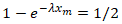 .
.
The following algebraic transformations will provide the answer.
| For the median, the left-tail probability is the same as the right-tail one. | |
| The natural logarithms of both sides are also equal. | |
| We simplified the left side based on the fact the the natural logrithm is an inverse for the expenential functions, | |
| We get this by dividing both the sides by -λ. | |
| In this version we replaced 1/2 with 2-1 (see [Negative Exponents]). | |
| The Power Rule states that a·ln(b) = ln(ba); here -ln(2-1) =(-1)·ln(2-1)= ln(2(-1)·(-1)) = ln(2). |
2. The mode of a continuous random variable is such a value for which the density function takes on a maximum value [Letkowski, Wikipedia-Mode]. The Exponential density is a unimodal function having the highest value at x = 0. Thus the mode is equal to zero (xmod = 0).
The variance of the Exponential variable is the square of the mean:
The standard deviation is the square root of the variance:
So the mean (μ) and standard deviation (σ) are for the Exponential distribution the same.
So the mean (μ) and standard deviation (σ) are for the Exponential distribution the same.
Spreadsheet Implementation for the Exponential Density, CDF, and Percentile
R Implementation for the Exponential Density, CDF, and Percentile
Example - Exponential
Suppose that an electric bulb's life time is exponentially distributed with the mean, μ = 1000 hours.
| 1 | What is the probability that the bulb will work no longer than 500 hours? |
| 2 | How likely is it for the bulb to work exactly 1,000 hours? |
| 3 | What is the probability that the bulb will serve longer than 2,000 hours? |
| 4 | What is the probability that the bulb will work ±200 hours around the mean (μ)? |
| 5 | How likely is it for the bulb to work between 500 and 1,000 hours? |
| 6 | What is the probability that the bulb will operate no more than 500 and at least 2,000 hours? |
| 7 | How likely is it for the bulb to work no longer than 300 or longer than 300 hours? |
| 8 | What is the 2nd quartile (median) of the life-time of the bulb? |
| 9 | What is the expected value (μ) of the bulb's life-time? |
| 10 | What is the variance (σ2) of the bulb's life-time? |
| 11 | What is the standard deviation (σ) of the bulb's life-time? |
Solution
Spreadsheet Solution
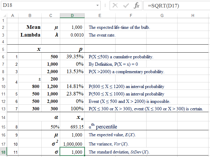
Formulas:
D6: =EXPON.DIST(C6,D3,TRUE)
D8: =1-EXPON.DIST(C8,D3,TRUE)
D10: =EXPON.DIST(C10,$D$3,TRUE)-EXPON.DIST(B10,$D$3,TRUE)
D11: =EXPON.DIST(C11,$D$3,TRUE)-EXPON.DIST(B11,$D$3,TRUE)
D15: =-LN(1 - C15) / D3
D16: =D2
D17: =D16^2
D18: =SQRT(D17)
This spreadshet solution is also available as an Excel workbook.
R Solution
# R Solutions
mu = 1000
lambda = 1/mu
# 1. The probability that the bulb will work no longer than 500 hours.
x = 500
p_upto500 = pexp(x, rate=lambda)
# In order to show a percentage value, it is first rounded to 2 decimal places.
# Next, using function paste the value is combined without a space with
# the percent sign. Function cat shows it all but it needs an explicit line
# line feed ("\n").
# It is complicated but it works well.
cat(paste(round(100*p_upto500, 2), "%", sep=""),"\n")
39.35%
# 2. The probability that the bulb will work exactly 1000 hours.
p_eq1000 = 0 # ... by definition
cat(paste(round(100*p_eq1000, 2), "%", sep=""),"\n")
0%
# 3. The probability that the bulb will serve longer than 2,000 hours?
x = 2000
p_above2000 = 1 - pexp(x, rate=lambda) # Same as pexp(x, rate=lambda, lower.tail = FALSE)
cat(paste(round(100*p_above2000, 2), "%", sep=""),"\n")
13.53%
# 4. The probability that the bulb will work ±200 hours around the mean (µ).
# ±200 hours around the mean means between 800 and 1,200.
delta = 200
x1 = mu - delta
x2 = mu + delta
p_between800and1200 = pexp(x2, rate=lambda) - pexp(x1, rate=lambda)
cat(paste(round(100*p_between800and1200, 2), "%", sep=""),"\n")
14.81%
# 5. The likelyhood for the bulb to work between 500 and 1,000 hours
x1 = 500
x2 = 1000
p_between500and1000 = pexp(x2, rate=lambda) - pexp(x1, rate=lambda)
cat(paste(round(100*p_between500and1000, 2), "%", sep=""),"\n")
23.87%
# 6. The probability that the bulb will operate no more than 500 and at least 2,000 hours
p_upto500andover2000 = 0
# This is a probability (0) of an impossible event.
# 7. The probability that the bulb to work no longer than 300 or longer than 300 hours?
p_upto300orabove300 = 1
# This is a probability (1) of a certain event. (X = 300) or (X > 300) covers all real numbers/
# 8. The 2nd quartile (median) of the life-time of the bulb.
alpha = 0.5
x_alpha = qexp(alpha, rate=lambda)
cat(x_alpha, "\n")
693.1472
# 9. The expected value.
cat(mu, "\n")
1000
# 10. The variance.
var = 1/lambda^2 # Same as mu^2.
cat(var, "\n")
1e+06
# 11. The standard deviation.
stdev = sqrt(var)
cat(stdev, "\n")
1000
Remarks
| 1 |
The probability that the bulb will work no longer than 500 hours is the cumulative probability for any time up to 500 hours, P(T ≤ 500) = 39.35%. This solution uses the Left-tail Probability Pattern. Spreadsheet formula is =EXPON.DIST(500,0.001,TRUE). R formula is pexp(500, rate=0.001). |
| 2 | The probability that the bulb will work exactly 1,000 hours is zero. The bulb's life time (T) is a continuous random variable. Recall that all point probabilities, P(T = t), are equal to zero for such variables. |
| 3 | To assess the probability that the bulb will serve longer than 2,000 hours we notice that event "longer than 2,000, (T > 2000)" is complementry to event "up to 2,000, (T ≤ 2000)". Therefore, based on the Law of Addition, we have P(T > 2000) = 1 - P(T ≤ 2000) = 13.53%. This solution uses the Right-tail Probability Pattern. Spreadsheet formula is =1 - EXPON.DIST(2000,0.001,TRUE). R formula is 1 - pexp(2000, rate=0.001) which is the same as pexp(2000, rate=0.001, lower.tail = FALSE). |
| 4 |
The probability that the bulb will work ±200 hours around the mean (μ). Since μ = 1000, this statement is equivalent to the life-time of the bulb being between 800 and 1200. Thus using, the Interval Probability Pattern. we have: P(800 ≤ T ≤ 1200) = P(T ≤ 1200) - P(T ≤ 800) = 14.81%. Spreadsheet formula is =EXPON.DIST(1200,0.001,TRUE) - EXPON.DIST(800,0.001,TRUE). R formula is pexp(1200, rate=0.001) - pexp(800, rate=0.001). |
| 5 |
The likelyhood for the bulb to work between 500 and 1,000 hours. This case is similar to the above (4), P(500 ≤ T ≤ 1000) = P(T ≤ 1000) - P(T ≤500) == 23.87%. Spreadsheet formula is =EXPON.DIST(1000,0.001,TRUE) - EXPON.DIST(500,0.001,TRUE). R formula is pexp(1000, rate=0.001) - pexp(500, rate=0.001). |
| 6 | The probability that the bulb will operate no more than 500 AND at least 2,000 hours is equal to zero. Event "no more than 500 AND at least 2,000" is an impossible event: (T ≤ 500) AND (T ≥ 2000). No T can be in the same time ≤ 500 AND≥ 2000. Thus (T ≤ 500) AND (T ≥ 2000) = 0. |
| 7 |
The likelyhood for the bulb to work no longer than 300 OR longer than 300 hours is one. Event "no longer than 300 OR longer than 300" is certain, (T ≤ 300) OR (T > 300). There are no life-times that wouldn't satisfy this event. This event covers all real numbers, ℝ.Thus P (T ≤ 300) OR (T > 300) = 1. |
| 8 |
The 2nd quartile (median) of the life-time of the bulb is such a value, tα, for which P(T ≤tα) = α, where α = 0.5. Using the Precentile formula we get tα ≈ 693.1472. Spreadsheet formula is =-LN(1 - 0.5) / 0.001). R formula is qexp(0.5, rate=0.001). |
| 9 | The expected value (μ) of the bulb's life-time is 1,000. Based on the definition of the expected value, E(X) = μ = 1/λ = 1,000. |
| 10 | The variance (σ2) of the bulb's life-time is 1,000,000. Based on the definition of the variance, Var(X) =σ2= 1/λ2 = 1,000,000. |
| 11 | The standard deviation (σ) of the bulb's life-time is 1,000. Based on the definition of the expected value, StDev(X) = σ = μ = 1,000. |
Q & A - Exponential Distribution
The time between arrivals of cars at Shining Body’s car-cleaning service follows an exponential probability distribution with a mean time between arrivals of 5 minutes. The management of this service would like to assess the following probabilities, percentiles, and expected parameters.
| 1 | What is the probability that the next car will arrive in less than 7 minutes? |
| 2 | How likely is it for the next car to drive in more than 4 minutes? |
| 3 | What is the probability that that the next car will arrive in between 3 and 6 minutes? |
| 4 | No car has arrived for 4 minutes since the arrival of the last car. What is the probability that the next car's arrival will not happen in the next 3 minutes. |
| 5 | What is the probability that that the next car will arrive in less than 4 or more than 7 minutes? |
| 6 | What is the probability that that the next car will arrive in less than 7 or more than 4 minutes? |
| 7 | How likely is it for the next car to drive in about 4 minutes (here about means ±30 seconds)? |
| 8 | Compare the probabilities of the inter-arrival times in intervals [0,1), [1,2), and [2,3), all in minutes. |
| 9 | What is the 90th percentile of the inter-arrival time? |
| 10 | What is the top 10th percentile of the inter-arrival time? |
| 11 | What is the expected value (μ) of the inter-arrival time? |
| 12 | What is the variance (σ2) of the inter-arrival time? |
| 13 | What is the standard deviation (σ) of the inter-arrival time? |
Solution
Spreadsheet Solution
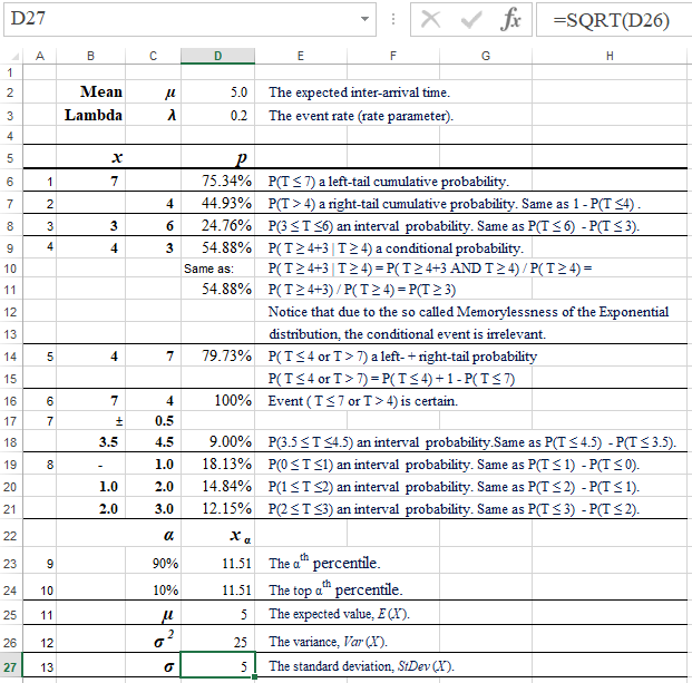
Formulas:
D6: =EXPON.DIST(B6,D3,TRUE)
D7: =1-EXPON.DIST(C7,D3,TRUE)
D8: =EXPON.DIST(C8,D3,TRUE)-EXPON.DIST(B8,D3,TRUE)
D9: =(1-EXPON.DIST(B9+C9,D3,TRUE))/(1-EXPON.DIST(B9,D3,TRUE))
D10: Same as:
D11: =1-EXPON.DIST(C9,D3,TRUE)
D14: =EXPON.DIST(B14,$D$3,TRUE)+1-EXPON.DIST(C14,$D$3,TRUE)
D18: =EXPON.DIST(C18,D3,TRUE)-EXPON.DIST(B18,D3,TRUE)
D19: =EXPON.DIST(C19,$D$3,TRUE)-EXPON.DIST(B19,$D$3,TRUE)
D20: =EXPON.DIST(C20,$D$3,TRUE)-EXPON.DIST(B20,$D$3,TRUE)
D21: =EXPON.DIST(C21,$D$3,TRUE)-EXPON.DIST(B21,$D$3,TRUE)
D23: =-LN(1 - C23) / D3
D24: =-LN(C24) / D3
D25: =D2
D26: =D25^2
D27: =SQRT(D26)
This spreadshet solution is also available as an Excel workbook.
R Solution
# R Statements
mu = 5
lambda = 1/mu
# 1. The probability of the inter-arrival time to be up to 7 minutes.
t = 7
p_upto7 = pexp(t, rate=lambda)
# In order to show a percentage value, it is first rounded to 2 decimal places.
# Next, using function paste the value is combined without a space with
# the percent sign. Function cat shows it all but it needs an explicit line
# line feed ("\n").
# It is complicated but it works well.
cat(paste(round(100*p_upto7, 2), "%", sep=""),"\n")
75.34%
# 2. The probability of the inter-arrival time to be longer than 7 minutes.
t = 4
p_above4 = 1 - pexp(t, rate=lambda)
cat(paste(round(100*p_above4, 2), "%", sep=""),"\n")
44.93%
# 3. The probability of the time to be between 3 and 6 minutes?
t1 = 3
t2 = 6
p_between3and6 = pexp(t2, rate=lambda) - pexp(t1, rate=lambda)
cat(paste(round(100*p_between3and6, 2), "%", sep=""),"\n")
24.76%
# 4. This is a conditional probability, P( T = 4+3 | T = 4).
# P( T = 4+3 | T = 4) = P( T = 4+3 AND T = 4) / P( T = 4) =
# P( T = 4+3) / P( T = 4)
# Due to memorylessness of the Exponential distribution, this probabaility
# can be reduced to P(T = 3).
tc = 4
t = 3
p_above3_given_morethan4 = (1 - pexp(tc+t, rate=lambda)) / (1 - pexp(tc, rate=lambda))
cat(paste(round(100*p_above3_given_morethan4, 2), "%", sep=""),"\n")
54.88%
# This is the same as:
cat(paste(round(100*(1-pexp(t, rate=lambda)), 2), "%", sep=""),"\n")
54.88%
# 5. This is a right- + left-tail probability, P( T = 4 or T > 7).
t1 = 4
t2 = 7
p_upto4or_above7 = pexp(t1, rate=lambda) + (1 - pexp(t2, rate=lambda))
cat(paste(round(100*p_upto4or_above7, 2), "%", sep=""),"\n")
79.73%
#6. Event ( T = 7 or T > 4) is certain.
p_upto7or_above4 = 1
cat(paste(round(100*p_upto7or_above4, 2), "%", sep=""),"\n")
100%
# 7. The probability for the time to be within 30 second of 4 minutes
delta = 30/60
t1 = 4 - d100%elta
t2 = 4 + delta
p_within30sec_of4 = pexp(t2, rate=lambda) - pexp(t1, rate=lambda)
cat(paste(round(100*p_within30sec_of4, 2), "%", sep=""),"\n")
9%
# 8. Interval probabilities, P(0 = T =1), P(1 = T =2), P(2 = T =3).
t1 = c(0,1,2)
t2 = t1 + 1
pexp(t2, rate=lambda) - pexp(t1, rate=lambda)
[1] 0.1812692 0.1484107 0.1215084
# Notice that the 1st probability id the highest because it interval is adjecent
# to the mode (0).
# 9. The 90th percentile.
alpha = 0.9
q_90 = qexp(alpha, rate=lambda)
cat(q_90,"\n")
11.51293
#10. The top 10th percentile (same as the 90th percentile).
alpha = 0.1
tq_10 = qexp(1-alpha, rate=lambda)
cat(tq_10,"\n")
11.51293
#11. The expected value, E(X).
cat(mu,"\n")
5
#12. The variance, Var(X).
cat(mu^2,"\n")
25
# 13. The standard deviation, StDev(X).
cat(mu,"\n")
5
Remarks
| 1 |
The probability that the next car will arrive in less than 7 minutes is the cumulative probability for any time up to 7 minutes, P(T < 7) = 39.35%. This solution uses the Left-tail Probability Pattern. Notice that, bacause T is a continuous variable, we have: P(T < 7) = P(T ≤ 7). Spreadsheet and R formulas: |
| 2 |
The likelihood for the next car to arrive in more than 4 minutes. This is a right-tail probability, P(T > 4) = 1 - P(T ≤ 4) = 44.93%. This solution uses the Right-tail Probability Pattern. Spreadsheet and R formulas: |
| 3 |
The probability that that the next car will arrive in between 3 and 6 minutes. This is an interval probability, P(3 ≤ T ≤ 6) = P(T ≤ 6) - P(T ≤ 3) = 24.76%. This solution uses the Interval Probability Pattern. Spreadsheet and R formulas: |
| 4 |
The probability that the next car will not arrive in the next 3 minutes, given already 4 minutes have elapsed since the last car's arrival. This is a conditional probability (see Multiplication Law): P(T > 4+3 | T > 4) a conditional probability. P( T > 4+3 | T > 4) = P( T > 4+3 AND T > 4) /P( T > 4) = P(T > 4+3) / P(T > 4) = 54.88%. Notice that due to the so called memorylessness of the Exponential distribution, the conditional event is irrelevant. Thus the [simpler] solution is P(T > 3). Based on the Event Intersection rule, the joint events (T > 4+3) and (T > 4) are reduced to (T > 4+3). 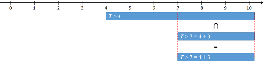 Event (T = 4+3) is contained in event (T > 4). This is why P(T > 4+3 AND T > 4) = P(T > 4+3). Spreadsheet and R formulas: |
| 5 |
The probability that that the next car will arrive in less than 4 or more than 7 minutes?
This is a left- + right-tail probability, P(T < 4 OR T > 7) = 79.73%. This solution uses both the Left-Tail and Right-Tail patterns.
Spreadsheet and R formulas: |
| 6 |
The probability that that the next car will arrive in less than 7 or more than 4 minutes is one. 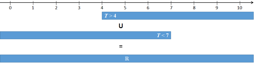 Event (T < 7 or T > 4) is certain. Thus P(T < 7 or T > 4) = 100%. |
| 7 |
The likelihood for the next car to drive in about 4 minutes ±30 seconds is
P(3.5 ≤ T ≤ 4.5) = P(T ≤ 4.5) - P(T ≤ 3.5) = 9%. This solution uses the Interval Probability Pattern.
Spreadsheet and R formulas: |
| 8 |
Compare the probabilities of the inter-arrival times in intervals [0,1), [1,2), and [2,3), all in minutes. All these probabilities apply the Interval Probability Pattern, P(T ∈[0,1)) = 18.13%, P(T ∈[1,2)) = 14.84%, and P(T ∈[2,3)) = 12.15%.
Spreadsheet and R formulas: t1 = c(0,1,2) t2 = t1 + 1 pexp(t2, rate=0.2) - pexp(t1, rate=0.2) (The last one returns a vector of the three probabilities in question.) |
| 9 |
The 90th percentile of the inter-arrival time is such a value, tα,
for which the left-tail probability is α = 0.9, P(T ≤ tα) = α,
tα = 11.51293. Spreadsheet and R formulas: |
| 10 |
The top 10th percentile of the inter-arrival time is such a value, t1-α,
for which the right-tail probability is α = 0.1, P(T > t1-α) = α, t1-α = 11.51293. Spreadsheet and R formulas: |
| 11 | The expected value (μ) of the inter-arrival time is 1/λ = 5. |
| 12 | The variance (σ2) of the inter-arrival time is 1/λ2 = 25. |
| 13 | The standard deviation (σ) of the inter-arrival time is μ = 5. |
"Normal distributions are important in statistics and are often used in the natural and social sciences to represent real-valued random variables whose distributions are not known. Their importance is partly due to the central limit theorem. It states that, under some conditions, the average of many samples (observations) of a random variable with finite mean and variance is itself a random variable whose distribution converges to a normal distribution as the number of samples increases. Therefore, physical quantities that are expected to be the sum of many independent processes (such as measurement errors) often have distributions that are nearly normal." [Wikipedia-Normal]
- A common shortcut for the Normal distribution with parameters µ and σ is N(μ,σ). We say, a random variable X, having distribution N(μ,σ), is Normally distributed with the mean of μ and standard deviation σ. Another symbolic way to indicate that a random variable is normally distributed is though shortcut Xμσ.
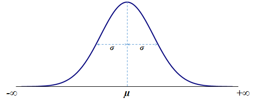
- The Normal probability distribution is the most important distribution for describing and analyzing continuous random variables. Its density function is probably best known as a bell shaped curve.
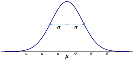
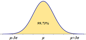
The standard deviation (σ) represents the distance from the mean (μ) to each of the inflexion points (marked up by the small circles). Also, the area under the curve (probability) within the interval of three standard deviations around the mean, (μ-3·σ, μ+3·σ) accounts for approximately 99.73%—the 3σ empirical rule:
P(μ-3·σ ≤ X ≤ μ+3·σ) ≅ 99.73%
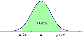
Other σ rules (so called empirical rules) state (the 2σ empiricalrule):
P(μ-2·σ ≤ X ≤ μ+2·σ) ≅ 95.45%
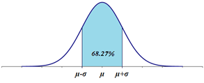
and (the 1σ empirical rule):
P(μ-1·σ ≤ X ≤ μ+1·σ) ≅ 68.27%
In other words, in a Normal population, there are approximately 99.73% of data within three standard deviations of the mean, 95.4%—within two standard deviations of the mean, and 68.27%—within one standard deviations of the mean. - The Normal probability distribution is used in a wide variety of applications including: heights of people, sitting heights (from the seat level to the head's top), rainfall amounts, test scores, industrial & scientific measurements, observational errors, etc..
- It is also the continuous distribution with the maximum entropy for a specified mean and variance.
- Abraham de Moivre, a French mathematician, published The Doctrine of Chances in 1733 in which he introduced this distribution.
- The density function of the Normal distribution is also known as Gauss function in honor to one of the greatest mathematicians, Carl Friedrich Gauss, who contributed immensely to this distribution.
- It is widely used in statistical inference (mainly as the distribution of the sample mean).
The domain of Normal random variables is the set of all Real numbers, X ∈ ℝ (-∞,+∞). Formally, the Normal distribution, N(μ,σ), is defined by the following density function:
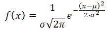
There is no close-form function, resulting from integration of this density function. However, most of the statistical software programs are equipped with precise numerical algorithms to do this job (see spreadsheet and R formulas below).
The αth percentile (quantile), xα, is the value of the inverse of the cdf, F(xα) = P(Xμσ≤ xα). This is such a value, xα, for which the cumulative probability is equal to α. In short, we write: P(Xμσ≤ xα) = α then xα is the αth percentile (quantile) or:
xα = F-1(α)
Again, since there is no close-form function for this inverse function, the percentiles are calculated numerically (see spreadsheet and R formulas below).
The expected value (mean) of the Normal variable is equal to the μ parameter of this distribution.
The standard deviation of the Normal variable is equal to the σ parameter of this distribution.
The variance of the Normal variable is just σ2
Example - Normal Parameters
For a Normally distributed random variable, X: N(100,20), the expected value E(X) = 100, the variance Var(X) = 400, and the standard deviation StDev(X) = 20.
There is a special version of the Normal distribution, referred to as the Standard Normal distribution. This distribution has the mean (μ) and standard deviation (σ) equal to 0 and 1, respectively. It random variable is commonly named as Z. Its density, f(z), and cdf, F(z), functions are simpler but still to complex for calculus operations.
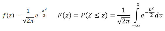
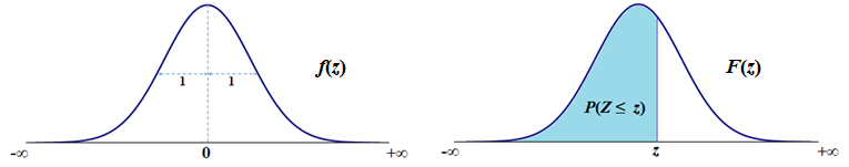
This special version of the Normal distribution used to be more relevant when there were no computer-based solutions to assess Normal probabilities. Such assessments were done, using tabulated Normal probabilities for selected value of the Standard Normal variable (Z). Our ability to figure out probabilities and percentiles based on the results obtained for the Standard Normal variables is grounded in a simple relationship between General Normal and Standard Normal variables:
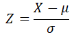
If X has distribution N(μ, σ), then Z has standard distribution N(0, 1):


Examples - Normal Transformations
Suppose that we want to assess a left-tail probability, P(X≤75), for Normal distribution N(100, 25). Using the Z transformation, (75 - 100)/25 = -1, we need to find out P(Z≤-1). This is the cumulative probability that we find in the table for the negative Z values, in the row of -1.0 and column 0.00:
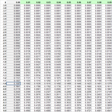
Thus P(Z ≤ -1) ≅ 0.1587 ≅ P(X ≤ 75). There is about 15.87% chance for X to be up to 75. This outcome can also be derived from the one σ - empirical rule, according to which P(μ-σ ≤ X ≤ μ+σ) ≅ 68.27%.
Plugging in μ = 100, and σ = 25, we get P(100-25 ≤ X ≤ 100+25) = P(75 ≤ X ≤ 125)≅ 68.27%.
Notice that event (75 ≤ X ≤ 125) complementaty to event (X < 75 or X > 125). Therefore P(X < 75 or X > 125) = 1 - P(75 ≤ X ≤ 125) ≅ 100% - 68.27% = 31.73%. Due the symmetry of the Normal distribution, P(X < 75 or X > 125) = 2 · P(X < 75) ≅ 31.73%. We finnaly get P(X < 75) ≅ 31.73% / 2≅15.87%. In particular, this solution is correct since the end-points (75 and 125) are one standard deviation (σ = 25) below and above the mean (μ = 100), respectively.
Next, how can we find out a right-tail probability, P(X > 131.25), for Normal distribution N(100, 25). Using the Z transformation, (131.25 - 100)/25 = 1.25, we need to find out P(Z > 1.25). Notice that P(Z > 1.25) = 1 - P(Z ≤ 1.25). We can find probability from the Standard Normal table for the non-negative values of Z in the row of 1.2 and column 0.05 (1.2 + 0.05 = 1.25):
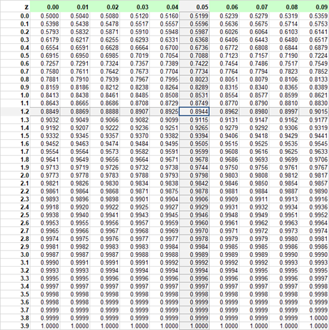
Thus P(Z ≤ 1.25) ≅ 0.8944. Ultimately we need P(Z > 1.25) ≅ 1 - 0.8944 = 0.1056 ≅ P(X > 131.25). There is about 10.56% chance for X to be greater than 131.25.
The above Empirical Rule examples are relatively simple. We were able to find exact match for the Z values (with the two-decimal-digit precision).
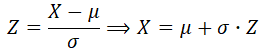
Let's do a little more complicated case. Suppose that we want to find the third quartile (75th percentile) for this distribution, N(100, 25). If we can find the third quartile (75th percentile) for the Standard Normal ditribution, N(0, 1), then we can transform it to X as follows:
Let's do a little more complicated case. Suppose that we want to find the third quartile (75th percentile) for this distribution, N(100, 25). If we can find the third quartile (75th percentile) for the Standard Normal ditribution, N(0, 1), then we can transform it to X as follows:
In order to indentify the 75th percentile in the Standard Normal probability table, we need to first find the 0.75 probability inside the table.
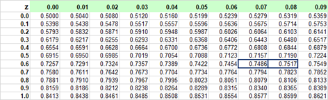
Unfortunatley, there is no exact match for probability 0.75. The closest values are 0.7486 and 0.7517. Cumulative Probability 0.75 is close to a half-way between 0.7486 and 0.7517.
Averaging the Z values (0.67, 0.68) associated with these probabilities, we get an approximate solution:
P(Z < z) = 0.75 ⇒ z ≅ (0.67+0.68)/2 = 0.675. Using the transformation formula, we finnaly get:
P(X < x) = 0.75 ⇒ x ≅ μ + z · σ = 100 +0.675 · 25 = 116.875.
The normal variable value of approximately 116.875 is the third quartile for distribution N(100, 25).
P(Z < z) = 0.75 ⇒ z ≅ (0.67+0.68)/2 = 0.675. Using the transformation formula, we finnaly get:
P(X < x) = 0.75 ⇒ x ≅ μ + z · σ = 100 +0.675 · 25 = 116.875.
The normal variable value of approximately 116.875 is the third quartile for distribution N(100, 25).
Note:
As you could see, using the probability tables can be complicated, confusing, and not accurate.
One has to be irrational, to it this stuff in such a convoluted way, especially while much simpler solutions are available. Using Spreadsheet or R functions (shown below) it takes just one expression to get it done. For this particulat problem, we have:
Lessons Learned:
Software tools are, in most cases, simpler and easier to implement. Most of the probability tables can be replaced with functions built-in statistical programs such as Excel or R.
While the Normal probability tables are not needed at all, the relationship between the general Normal variable, X: N(μ, σ), and the Standard Normal variable, Z: N(0, 0), is of great importance. It is particularly applicable in the Inferential Statistics.
Probability distribution N(μ,σ):
Probability distribution N(0,1) - Standard:
R Implementation for Exponential Density, CDF, and Percentile
Probability distribution N(μ,σ):
Probability distribution N(0,1) - Standard:
Notice that in R, the names of the function are the same for distributions N(μ,σ) and N(0,1). This is because the default values of the mean and sd parameters are 0 and 1, respectively (if you do not write these parameters, R will assume that mean = 0 and sd = 1).
Example - Normal Distribution
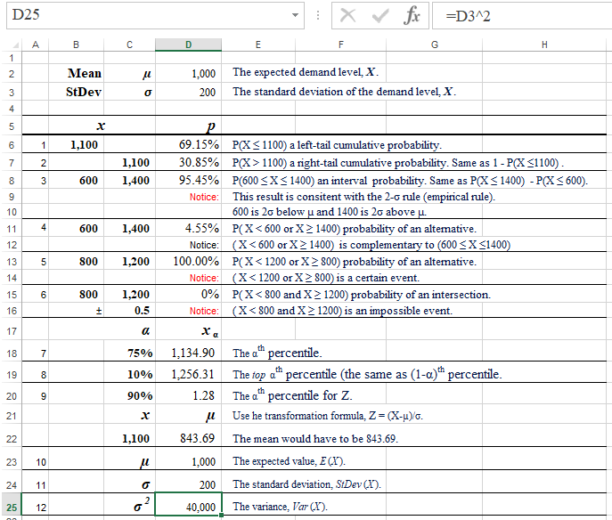
Given the daily demand, X, for some product has a normal distribution with the mean, μ =1,000, and the standard deviation, σ = 200, answer the following questions:
| 1 | What is the probability that demand X will be up to 1,100? |
| 2 | What is the probability of demand X to be greater than 1,100? |
| 3 | What is the probability of demand X to be between 600 and 1,400? |
| 4 | What is the probability of demand X to be lower than 600 or higher than 1,400? |
| 5 | What is the probability of demand X to be lower than 1,200 or higher than 800? |
| 6 | What is the probability of demand X to be lower than 800 and higher than 1,200?? |
| 7 | What is the 3rd quartile of demand X? |
| 8 | What is the top 10th percentile (quantile) of demand X? |
| 9 | What would the mean (μ) have to be in order for P(X < 1,100) to be 90% (σ = 200)? |
| 10 | What is the expected value of X, E(X)? |
| 11 | What is the standard deviation of X, StDev(X)? |
| 12 | What is the variance of X, Var(X)? |
Solution
Spreadsheet Solution
This spreadshet solution is also available as an Excel workbook.
Formulas:
D6: =NORM.DIST(B6,D2,D3,TRUE)
D7: =1-D6
D8: =NORM.DIST(C8,D2,D3,TRUE)-NORM.DIST(B8,D2,D3,TRUE)
D11: =1-D8
D13: 1
D15: 0
D18: =NORM.INV(C18,D2,D3)
D19: =NORM.INV(1-C19,D2,D3)
D20: =NORM.S.INV(C20)
D22: =C22-D20*D3
D23: =D2
D24: =D3
D25: =D3^2
R Solution
# R Solutions
mu = 1000
sigma = 200
# 1. The probability that demand X will be up to 1,100 (a left-tail probability).
x = 1100
p_upto1100 = pnorm(x, mean=mu, sd=sigma)
# In order to show a percentage value, it is first rounded to 2 decimal places.
# Next, using function paste the value is combined without a space with
# the percent sign. Function cat shows it all but it needs an explicit line
# line feed ("\n").
# It is complicated but it works well.
cat(paste(round(100*p_upto1100, 2), "%", sep=""),"\n")
69.15%
# 2. The the probability of demand X to be greater than 1,100 (a right-tail probability).
# Notice that event (X > 1100) is complementary to (X <= 1100).
# In R you can consider this also in this way:
# pnorm(x, mean=mu, sd=sigma, lower.tail = FALSE)
x = 1100
p_above1100 = 1 - pnorm(x, mean=mu, sd=sigma)
cat(paste(round(100*p_above1100, 2), "%", sep=""),"\n")
30.85%
# 3. The probability of demand X to be between 600 and 1,400, (600 <= X <=1400).
x1 = 600
x2 = 1400
p_between600and1400 = pnorm(x2, mean=mu, sd=sigma) - pnorm(x1, mean=mu, sd=sigma)
cat(paste(round(100*p_between600and1400, 2), "%", sep=""),"\n")
95.45%
# 4. The probability of demand X to be lower than 600 or higher than 1,400.
# Adopt the answers to questions 1 and 2 or take advantage of the answer to
# question 3 by noticing that (X < 600) OR (X > 1400) is complementary of
# (600 <= X <= 1400).
p_below600_or_above1400 = 1 - p_between600and1400
cat(paste(round(100*p_below600_or_above1400, 2), "%", sep=""),"\n")
4.55%
# This is the same as:
cat(paste(round(100*(pnorm(x1, mean=mu, sd=sigma) + 1 - pnorm(x2, mean=mu, sd=sigma) ), 2), "%", sep=""),"\n")
4.55%
# 5. The probability of demand X to be lower than 1,200 or higher than 800.
# Event X < 1200 OR X > 800 is certain.
p_below1200_or_above800 = 1
cat(paste(round(100*p_below1200_or_above800, 2), "%", sep=""),"\n")
100%
# 6. The probability of demand X to be lower than 800 and higher than 1,200.
# Event X < 800 AND X > 1200 is impossible.
p_below800_and_above1200 = 0
cat(paste(round(100*p_below800_and_above1200, 2), "%", sep=""),"\n")
# 7. The 3rd quartile of demand X.
alpha = 0.75
q_75th = qnorm(alpha, mean=mu, sd=sigma)
cat(q_75th,"\n")
1134.898
# 8. The top 10th percentile (quantile) of demand X.
alpha = 0.1
q_top10th = qnorm(1-alpha, mean=mu, sd=sigma)
cat(q_top10th,"\n")
1256.31
# 9. What would the mean (µ) have to be in order for P(X < 1,100) to be 90% (s = 200).
# Consider the Z-X transformation formula: Z = (X-µ)/s.
# We know X = 1100, sigma = 200, and a = 0.9. Having a, we can get Z as the ath percentile.
alpha = 0.9
x = 1100
zq_90th = qnorm(alpha) # By default mean = 0, sd = 1
mu_tobe = x - zq_90th * sigma
cat(mu_tobe,"\n")
843.6897
# 10. The expected value of X, E(X)?
cat(mu,"\n")
1000
# 11. The standard deviation, StDev(X).
cat(sigma,"\n")
200
# 12. The variance, Var(X).
cat(sigma^2,"\n")
40000
Remarks
| 1 |
The probability that demand X will be up to 1,100 is P(X ≤ 1100) = 69.15%. This solution uses the Left-Tail Probability pattern. 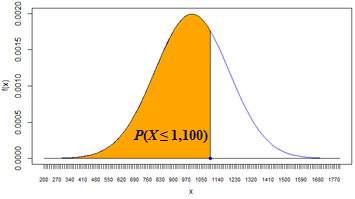
Spreadsheet and R formulas: |
| 2 |
The probability of demand X to be greater than 1,100 is P(X > 1100) = 30.85%. This solution uses the Right-Tail Probabililty pattern. 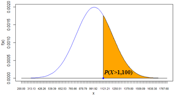 Spreadsheet and R formulas: |
| 3 | The probability of demand X to be between 600 and 1,400 is P(600 ≤ X ≤ 1,400) = 95.45%.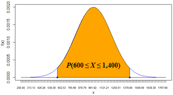 This solution uses the Interval Probabililty pattern. Also notice that this result is consitent with the 2-σ rule (empirical rule). The lower limit (600) is 2σ below the mean (μ=1000) and the upper limit (1,400) is 2σ above the mean. Spreadsheet and R formulas: |
| 4 | The probability of demand X to be lower than 600 or higher than 1,400 is P( X < 600 OR X > 1400) = 4.55%. 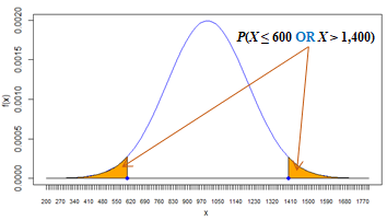 This is a complementary solution to that of #3 (4.55% = 100% - 95.45%) because event ( X < 600 OR X > 1400) is a complement of event (600 ≤ X ≤ 1,400). Spreadsheet and R formulas: |
| 5 | The probability of demand X to be lower than 1,200 or higher than 800 is 100%. Event ( X < 1,200 OR X > 800) is certain.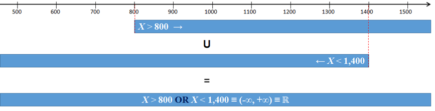 |
| 6 | The probability of demand X to be lower than 800 and higher than 1,200?
is 0%. Event ( X < 800 AND X > 1,200) is impossible, X < 800 AND X > 1,200 ≡ ∅.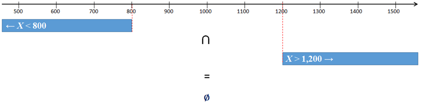 |
| 7 | The 3rd quartile of demand X is 1,134.90. This is the demand value for which P(X ≤ 1,134.90) = 75%.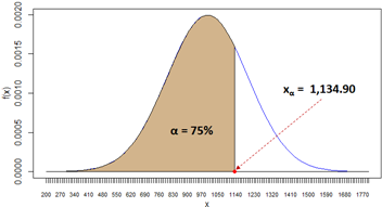 Spreadsheet and R formulas: |
| 8 | The top 10th percentile (quantile) of demand X is 1,256.31. This is the demand value for which P(X > 1,256.31) = 10%.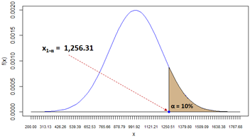 Spreadsheet and R formulas: |
| 9 |
What would the mean (μ) have to be in order for P(X < 1,100) to be 90% (σ = 200)? Notice that with the current mean (μ = 1,000), P(X < 1,100) = 69.15% (see the answer to question #1). For this probability to go up to 90%, the mean must be much smaller. This problem can be solved with a little help from the Standard Normal variable (Z), which is reated to the demand variable (X) as follows: From this formula we get: μ = X - z · σ. We only need the z value which is nothing else but the 90th percentile, zα, where α = 0.9, μ = X - zα· σ. Spreadsheet and R formulas: |
| 10 | The expected value of X, E(X) = μ = 1,000. |
| 11 | The standard deviation of X, StDev(X) = σ = 200. |
| 12 | The variance of X, Var(X)? = σ2 = 40,000. |
Q & A - Normal Distribution
From the bottle of Lifeway® Kefir:
"Kefir, known as the Champagne of Diary, has been enjoyed for over 2000 years. The probiotic cultures found in this bottle may help support immunity and healthy digestion and have contributed to the extensive folklore surrounding this beverage. Referred to in ancient texts, kefir is more than a probiotic superfood; kefir is a storied historic artifact."
"Kefir, known as the Champagne of Diary, has been enjoyed for over 2000 years. The probiotic cultures found in this bottle may help support immunity and healthy digestion and have contributed to the extensive folklore surrounding this beverage. Referred to in ancient texts, kefir is more than a probiotic superfood; kefir is a storied historic artifact."
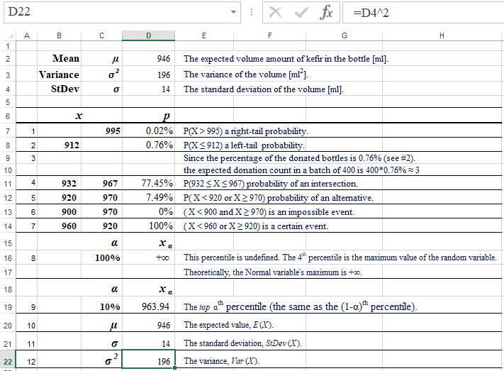
Kefir bottles are expected to contain 946 ml (approximately 1 quart) of cultured, lowfat milk (kefir). Quality control tests, performed regularly in the last 5 years, show quite stable variance of 196 ml2.
When solving the following problems, assume that the amount of kefir in the bottle is Normally distributed with μ = 946 ml, and variance σ2 = 196 ml2.
The maximum capacity of the bottle is 995 ml. If this capacity is exceed by the filling machine more than 5 times, the maching is stopped, inspected, and adjusted.
The management has set the standard for the minimum amount of kefir in 1 quart bottle to be 912 ml as well as for the prefect amount of kefir within the range of 932 to 967 ml.
Bottles containing less than 912 ml , if detected, are donated to the local elementry schools. The quality control engineer wants to assess some probabilities and percentiles related to the process of filling the bottles with kefir.
| 1 | What is the probability of overfilling a randomly selected bottle? |
| 2 | What is the probability that a randomly selected bottle will be donated? |
| 3 | From a batch of 400 bottles filled with kefir, how many are expected to be donated? |
| 4 | What is the probability that a randomly selected bottle will contain the perfect amount of kefir? |
| 5 | What is the probability of the amount of kefir, X, to be lower than 920 or higher than 970 ml? |
| 6 | What is the probability of the amount of kefir, X, to be lower than 900 and higher than 970 ml? |
| 7 | What is the probability of the amount of kefir, X, to be lower than 960 or higher than 920 ml? |
| 8 | What is the 4th quartile of the amount of kefir, X? |
| 9 | What is the top 10th percentile (quantile) of the amount of kefir, X? |
| 10 | What is the expected value of X, E(X)? |
| 11 | What is the standard deviation of X, StDev(X)? |
| 12 | What is the variance of X, Var(X)? |
Solution
Spreadsheet Solution
Formulas:
D4: =SQRT(D3)
D7: =1-NORM.DIST(C7,D2,D4,TRUE)
D8: =NORM.DIST(B8,D2,D4,TRUE)
D11: =NORM.DIST(C11,D2,D4,TRUE)-NORM.DIST(B11,D2,D4,TRUE)
D12: =1-(NORM.DIST(C12,D2,D4,TRUE)-NORM.DIST(B12,D2,D4,TRUE))
D13: 0
D14: 1
D19: =NORM.INV(1-C19,D2,D4)
D20: =D2
D21: =D4
D22: =D4^2
This spreadshet solution is also available as an Excel workbook.
# R Solutions
mu = 946
sigma = 14
# 1. The the probability of overfilling a randomly selected bottle, P(X > 995).
x = 995
p_above995 = 1 - pnorm(x, mean=mu, sd=sigma)
# In order to show a percentage value, it is first rounded to 2 decimal places.
# Next, using function paste the value is combined without a space with
# the percent sign. Function cat shows it all but it needs an explicit line
# line feed ("\n").
# It is complicated but it works well.
cat(paste(round(100*p_above995, 2), "%", sep=""),"\n")
0.02%
# 2. The probability that a randomly selected bottle will be donated.
# We are looking here for P(X ≤ 912).
x = 912
p_upto912 = pnorm(x, mean=mu, sd=sigma)
cat(paste(round(100*p_upto912, 2), "%", sep=""),"\n")
0.76%
# 3. From a batch of 400 bottles filled with kefir, how many are expected to be donated?
# This is the percentage of the donated bottles in the set of 400 bottles.
n = 400
expected_donated = p_upto912 * n
cat(expected_donated,"\n")
3.031688
# 4. The probability that a randomly selected bottle will contain the perfect amount of kefir.
# According to the standard the perfect amount is between 932 and 967.
# therefore the probability in question is P(932 ≤ X ≤ 967).
x1 = 932
x2 = 967
p_between932and967 = pnorm(x2, mean=mu, sd=sigma) - pnorm(x1, mean=mu, sd=sigma)
cat(paste(round(100*p_between932and967, 2), "%", sep=""),"\n")
77.45%
# 5. The probability of the amount of kefir, X, to be lower than 920 or higher than 970 ml
# This is the lower-tail (X < 920) probability + the upper-tail (X > 970) probability.
# Since the events are disjoint, P( X < 920 or X = 970) = P(X < 920) + P(X > 970).
x1 = 920
x2 = 970
p_below920_or_above970 = pnorm(x1, mean=mu, sd=sigma) + 1 - pnorm(x2, mean=mu, sd=sigma)
cat(paste(round(100*p_below920_or_above970, 2), "%", sep=""),"\n")
7.49%
# 6. The the probability of the amount of kefir, X, to be lower than 900 and higher than 970 ml
# Event (X < 900 AND X > 970) is impossible. Events (X < 900 ) and (X > 970) are disjoint.
# Their intersection is an empty set (impossible event).
p_below900_and_above970 = 0
cat(paste(round(100*p_below900_and_above970, 2), "%", sep=""),"\n")
0%
# 7. The probability of the amount of kefir, X, to be lower than 960 or higher than 920 ml.
# Event (X < 960 OR X > 920) is certain. All Real numbers satisfy this event.
# There are not Real numbers that wouldn't be below 960 OR above 920.
# (X < 960) OR ( X > 972) = (-8, +8).
p_below960_or_above920 = 1
cat(paste(round(100*p_below960_or_above920 , 2), "%", sep=""),"\n")
100.00%
# 8. The 4th quartile of the amount of kefir, X, is equivalent to the maximum value.
# Since the amount of kefir is Normally distributied, its theoretical maximum = +8.
# Therefore, this quartile is undefined or symbilically equal to +8.
# 9. The top 10th percentile (quantile) of the amount of kefir, X.
alpha = 0.1
q_top10th = qnorm(1-alpha, mean=mu, sd=sigma)
cat(q_top10th,"\n")
963.9417
# 10. This is a Normally distibuted random variable.
# It mean expected (value) is equal to paramter µ.
eX = mu
cat(eX,"\n")
946
# 11. The standard deviation of X, StDev(X), is equal to paramter s.
stDev = sigma
cat(stDev,"\n")
14
# 12. The variance of the amount of kefir, Var(X), is the square of the standard deviation.
var = sigma^2
cat(var,"\n")
196
Remarks
| 1 |
The probability of overfilling a randomly selected bottle, P(X > 995) = 0.02%. This solution uses the Right-Tail Probability pattern. This probability is so small that its area (to the right of point 995) can't be shown. 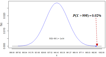 Spreadsheet and R formulas: |
| 2 |
The probability that a randomly selected bottle will be donated, P(X <= 912) = 0.76%. This solution uses the Left-Tail Probabililty pattern. 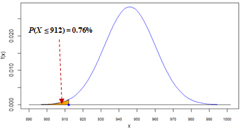 Spreadsheet and R formulas: |
| 3 |
From a batch of 400 bottles filled with kefir, how many are expected to be donated?. This is the percentage (0.76% - the answer to question #2) of the donated bottles in the set of 400 bottles. Approximately 3 (0.0076 * 400) bottles are expected to be donated from a batch of 400 bottles. |
| 4 |
The probability that a randomly selected bottle will contain the perfect amount of kefir. According to the management's standard, the perfect amount is between 932 and 967. Therefore the probability in question is P(932 ≤ X ≤ 967) = 77.45%. This solution is consistent with the Interval Probabililty pattern. 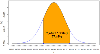 Spreadsheet and R formulas: |
| 5 |
The probability of the amount of kefir, X, to be lower than 920 or higher than 970 ml. This is a lower-tail (X < 920) probability + upper-tail (X > 970) probability. Since the events are disjoint, P(X < 920 or X > 970) = P(X < 920) + P(X > 970) = 7.49%. 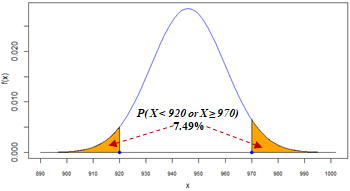 Spreadsheet and R formulas: |
| 6 |
The the probability of the amount of kefir, X, to be lower than 900 and higher than 970 ml. Event (X < 900 AND X > 970) is impossible. Events (X < 900 ) and (X > 970) are disjoint. Their intersection is an empty set (impossible event), (X < 900 ) AND (X > 970) = ∅. 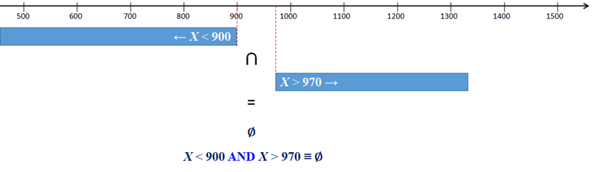 According to one of the probability rules, P(∅) = 0. |
| 7 |
The probability of the amount of kefir, X, to be lower than 960 or higher than 920 ml.
Event (X < 960 OR X > 920) is certain (S). All Real numbers satisfy this event.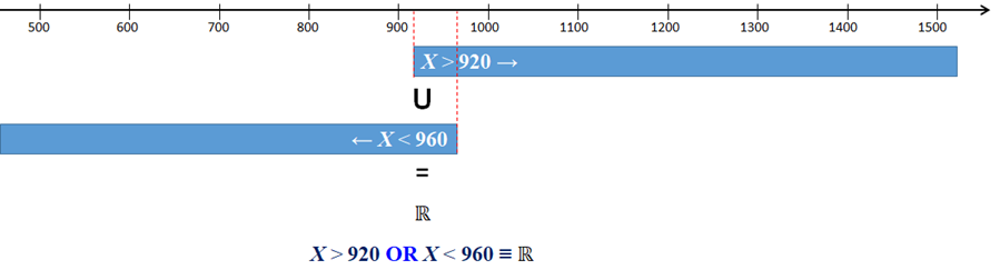 According to one of the probability rules, P(ℝ) = 1. (ℝ represents here a certain event). |
| 8 |
The 4th quartile of the amount of kefir, X, is equivalent to the maximum value of the random variable. Since the amount of kefir is Normally distributied, its theoretical maximum = +∞. Therefore, this quartile is undefined or symbilically equal to +∞. |
| 9 |
The top 10th percentile (quantile) of the amount of kefir, X, is 963.9417.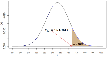 Spreadsheet and R formulas: |
| 10 | The expected value of X, E(X) = μ = 946. |
| 11 | The standard deviation of X, StDev(X) = σ = 14. |
| 12 | The variance of X, Var(X)? = σ2 = 196. |
Empirical - Coming Soon
References
| Brilliant (2020). Continuous Random Variables - Definition. URL-Source. | |
| Letkowski, J. (2013). In Search of the Most Likely Value. Journal of Case Studies in Education, Volume 5, Editor: Dr. Gina Almerico. | |
| Maths Is Fun (2020). Negative Exponents. URL-Source | |
| Maths Is Fun (2020). Working with Exponents and Logarithms. URL-Source | |
| Mun J. (2008). Understanding and Choosing the Right Probability Distributions. URL-Source | |
| Wikipedia-Central (2020). Central limit theorem. URL-Source | |
| Wikipedia-de Moivre (2020). Abraham de Moivre. URL-Source | |
| Wikipedia-Density (2020). Probability density function. URL-Source | |
| Wikipedia-Exponential (2020). Exponential distribution. URL-Source | |
| Wikipedia-Gauss (2020). Carl Friedrich Gauss. URL-Source | |
| Wikipedia-Mass-Function (2020). Probability mass function. URL-Source | |
| Wikipedia-Normal (2020). Normal distribution. URL-Source | |
| Wikipedia-Random Variable (2020). Random variable. URL-Source | |
| Wikipedia-Real Number (2020). Real number. Retrieved URL-Source. | |
| Wikipedia-Uniform (2020). Uniform distribution (continuous). URL-Source |